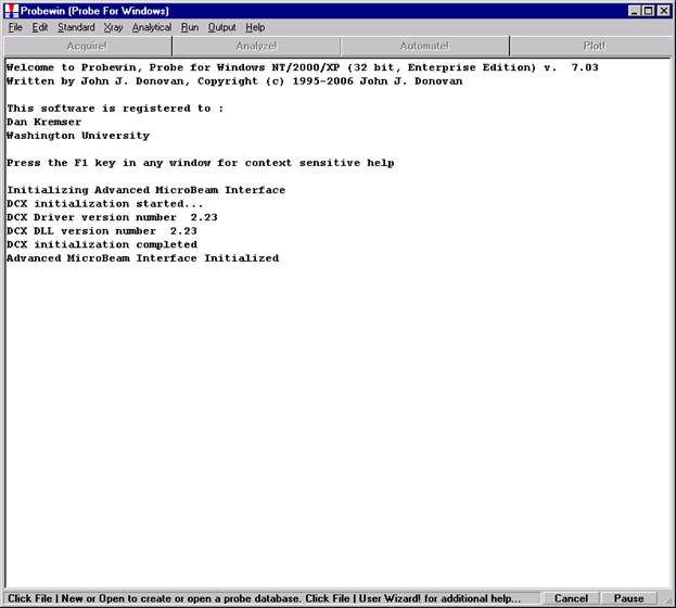
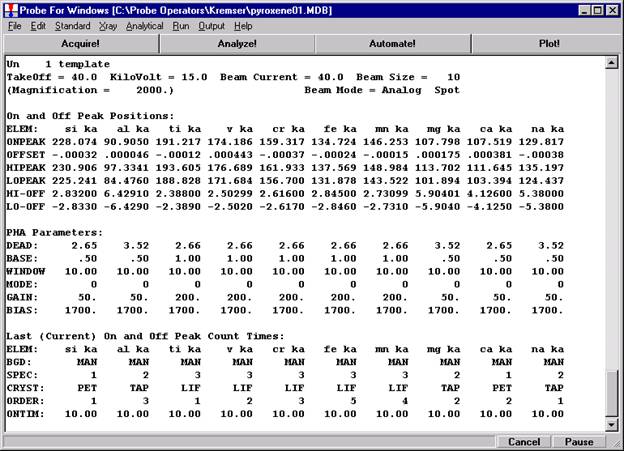
Probe for EPMA is a very versatile and powerful 32-bit acquisition, automation and analysis package for WDS and EDS electron microprobe analysis. This software (Probe for EPMA) is running under the Windows NT 4.0 (service pack 4) operating system on a Pentium PC platform.
One of the strengths of Probe for EPMA is the wide variety of options and features for many different tasks that are available to the probe operator. The aim of this manual then is to document some of the more advanced features usually skipped over in an introductory text. And as always, the path taken to cover a feature may not be the only avenue to approach the subject.
This manual was produced on the Washington University (Earth and Planetary Sciences) JEOL 733 Superprobe equipped with three wavelength dispersive spectrometers and using Probe for EPMA in demo mode.
Individual element analytical configurations for a specific element, x-ray, spectrometer, and reflecting crystal may be saved to the SETUP.MDB database for use in creating new sample setups within a probe run, for use in future runs or for documentation and performance evaluation purposes. The example below will illustrate how to create element setups from within a typical eight-element olivine routine and store them in a new SETUP.MDB database.
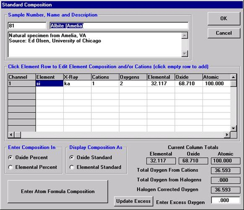
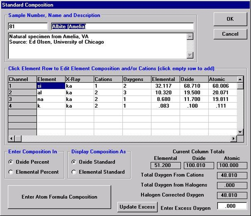
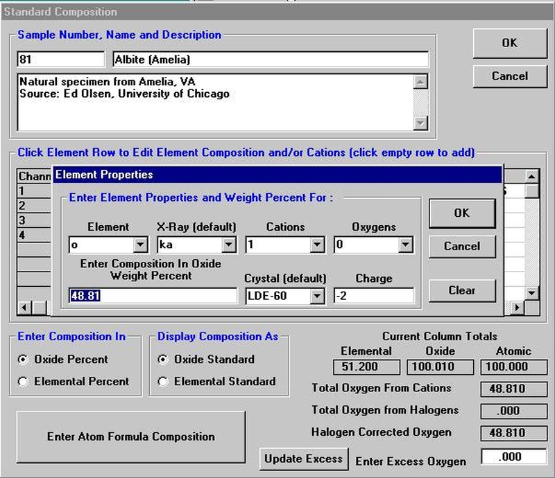
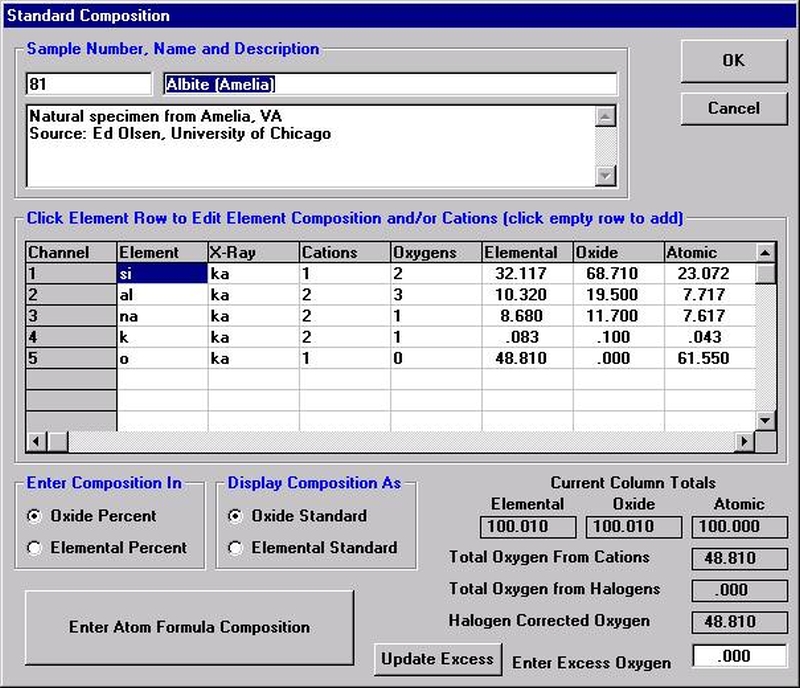
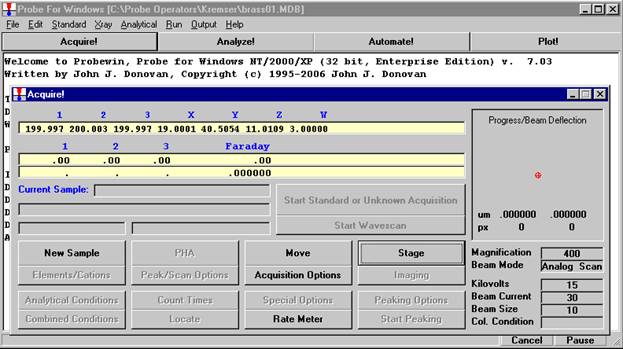
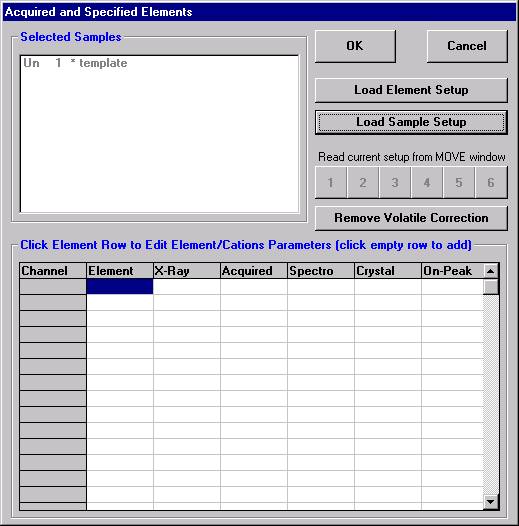
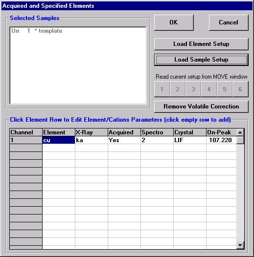
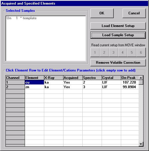
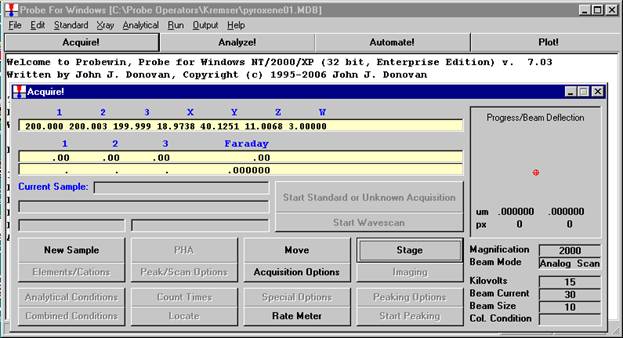
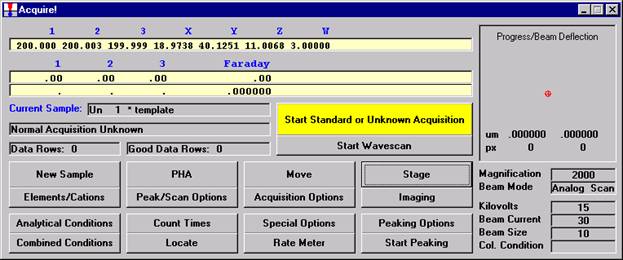
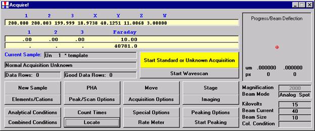
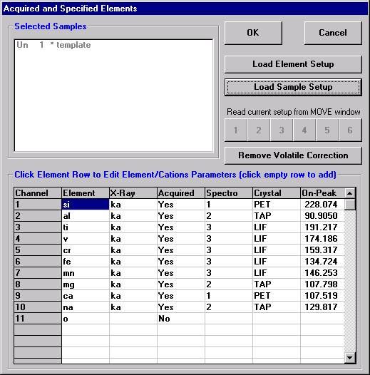
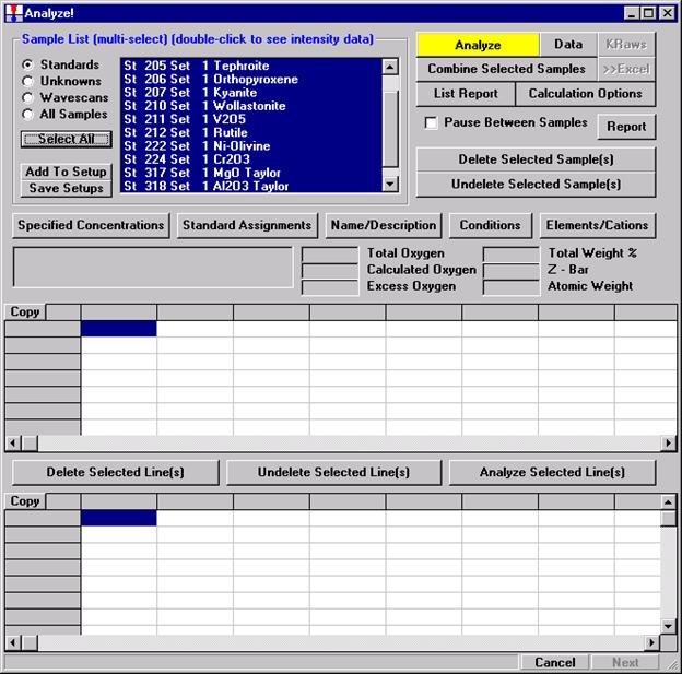
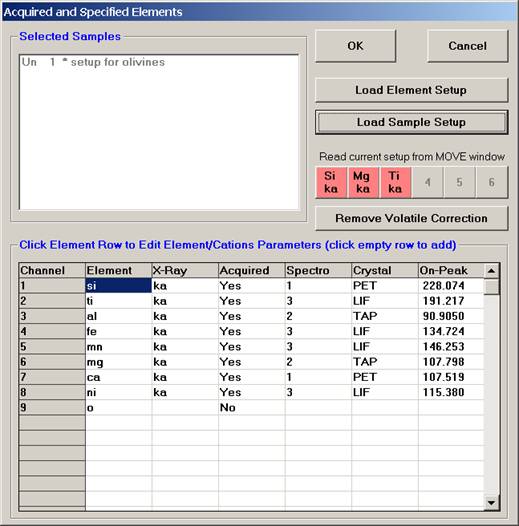
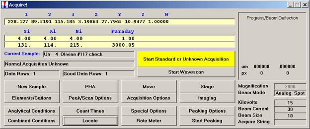
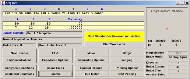
Open a new Probe for EPMA run in the usual manner. From the Acquire! window, create a new unknown sample from the New Sample dialog box, then click the Elements/Cations button. Next, enter the elements of interest into the Acquired and Specified Elements window in the usual manner. Below is the completed Acquired and Specified Elements window after the entry of all eight elements plus oxygen.
Go through the calibration process; find new peak positions and standardize to acquire intensity data on each standard. Normally one should save the element setup of an element that is assigned as the standard for that element. This is done because in that case the x-ray intensity data, P/B data, PHA parameters, and other information will also be saved in the SETUP.MDB database. This information is very useful for documentation and evaluation purposes.
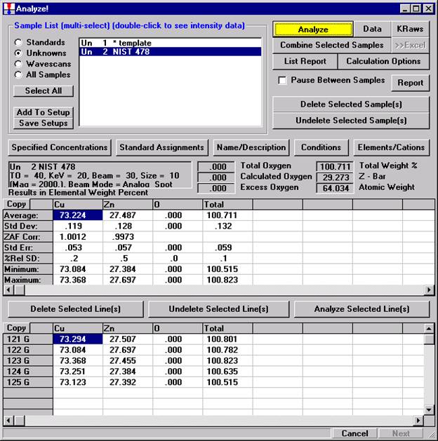
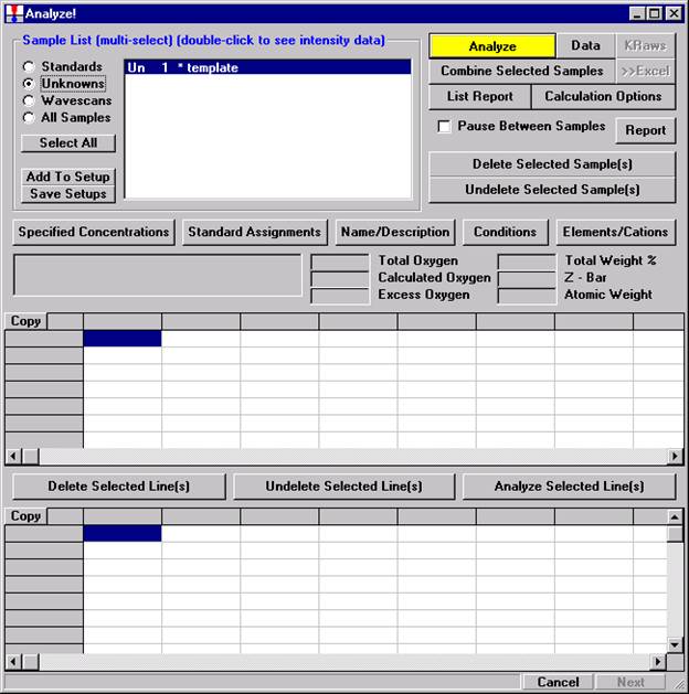
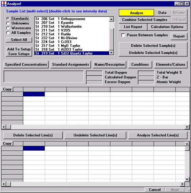
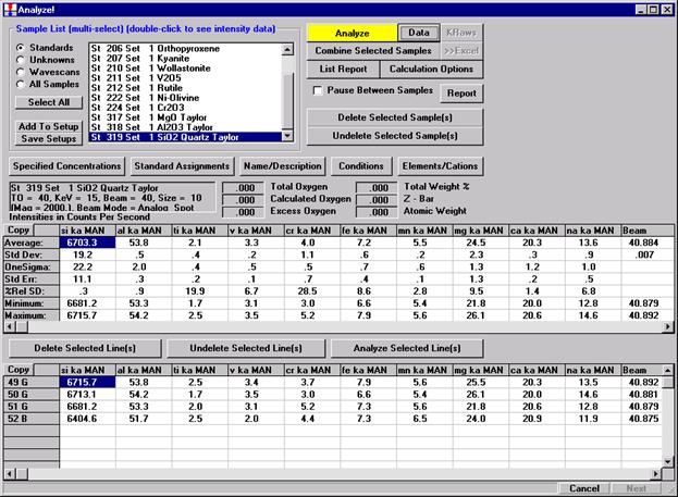
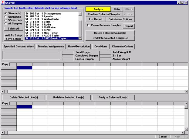
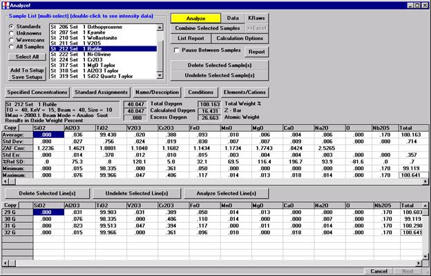
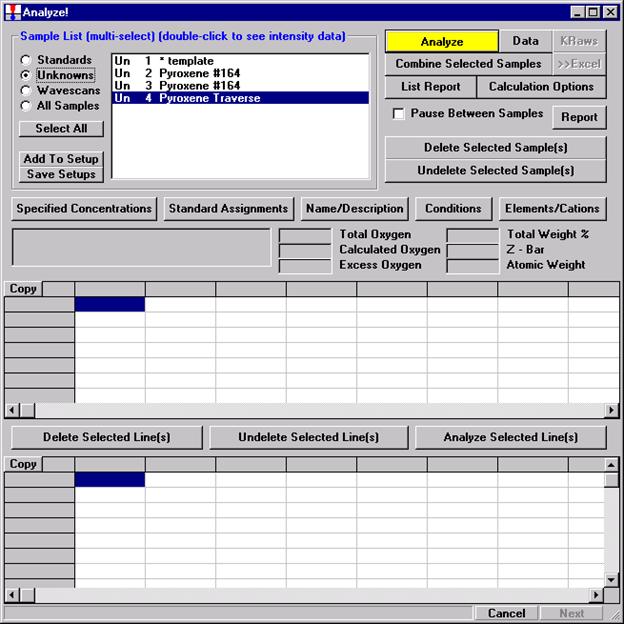
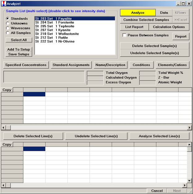
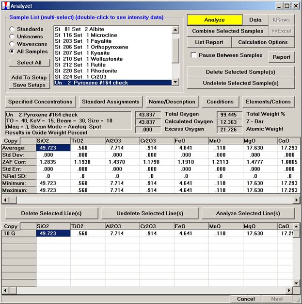
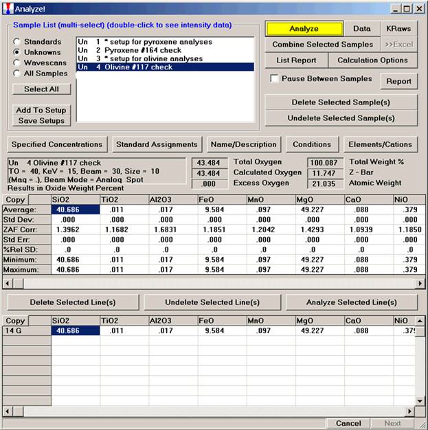
After completing the calibration and standardization process, open the Analyze! window. Choose the element setup to be stored and highlight the standard (iron in fayalite, in this example).
Click the Elements/Cations button.
This opens the Analyzed and Specified Elements window.
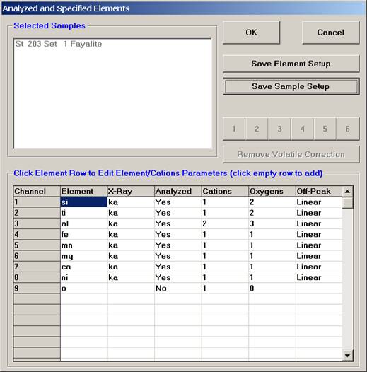
Click the Save Element Setup button.
The SetupOpenNewFile window will appear if no existing SETUP.MDB database exists.
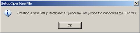
Click the OK button.
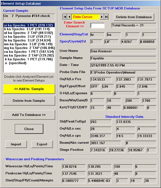
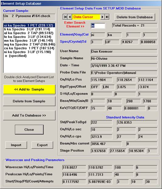
The Element Setup Database opens.
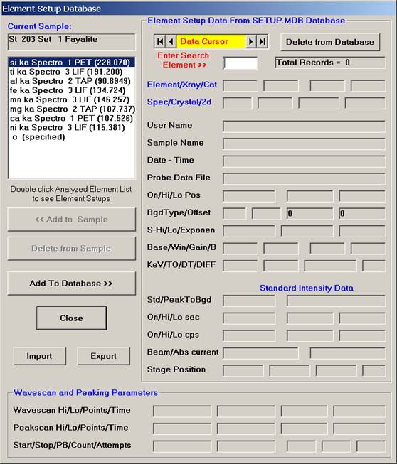
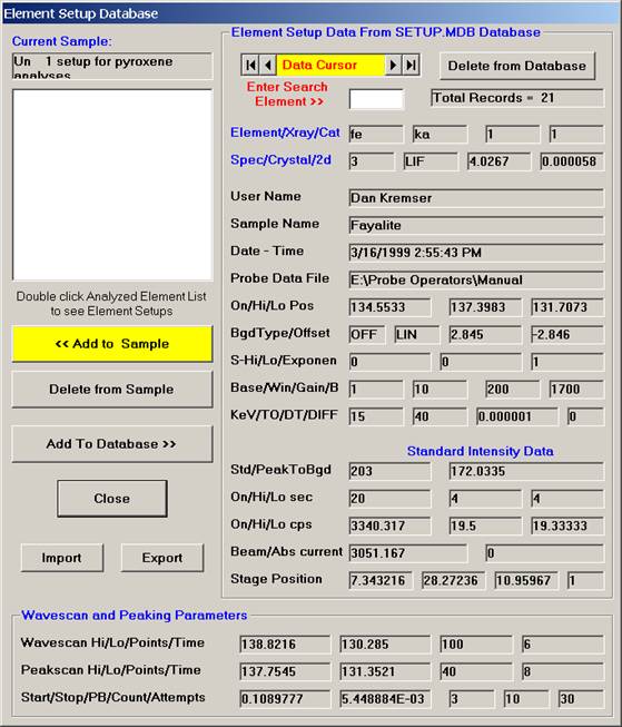
Highlight the specific element to save and click the Add To Database >> button. In this standard, the iron intensity is to be archived, select Fe kα Spectro 3 LIF (134.724).
Record number 1 has been stored as illustrated below. Note that the standard x-ray intensity and wavescan parameter data are stored as well.
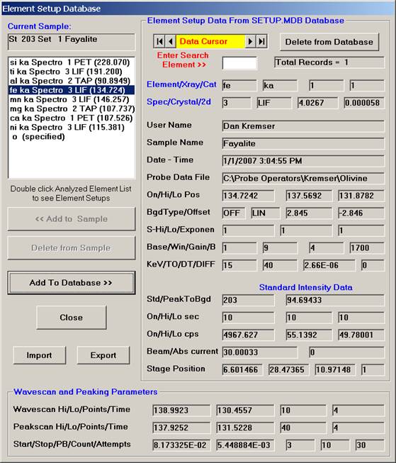
Click the Close button. The Analyzed and Specified Elements window reappears. Click the OK button. The Analyze! window returns.
The other element setups from this calibrated and standardized run or other probe runs may be entered into the database in a similar manner for future use.
To recall an element setup from the SETUP.MDB database for a new sample setup follow the procedure outlined below. Open a new PROBE FOR WINDOWS run. This process will also be applicable if the user simply wants to add an element to an existing sample setup. This example will illustrate recalling elements from the database for the setup of a new pyroxene run.
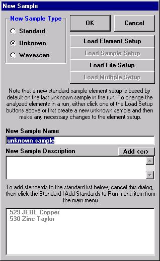
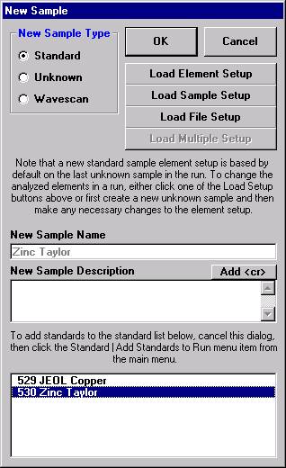
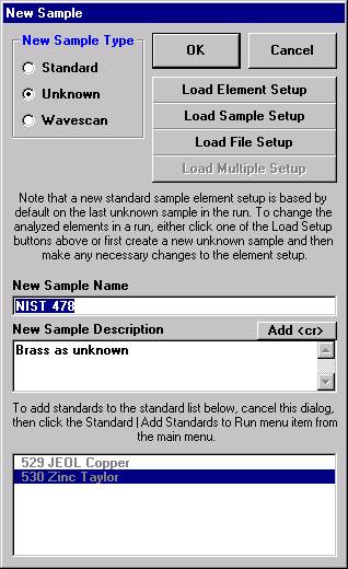
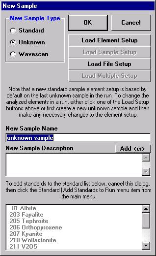
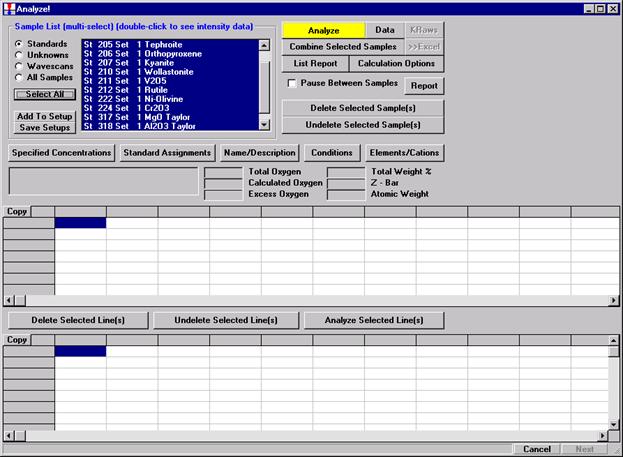
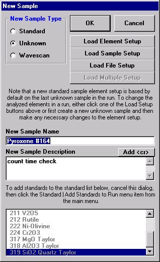
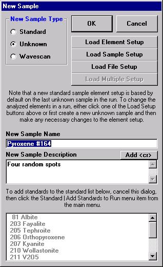
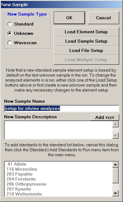
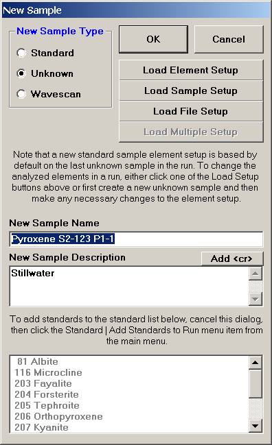
From the Acquire! window, click the New Sample button.
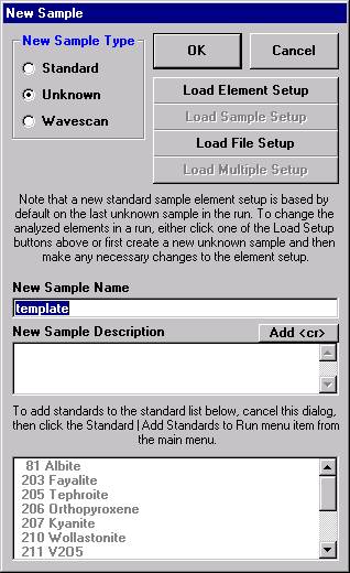
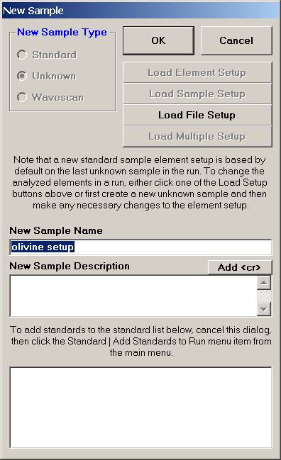
This opens the New Sample window. Edit the New Sample Name text field.
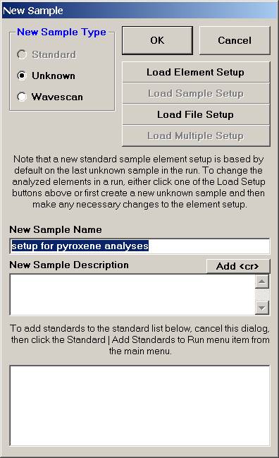
Click the Load Element Setup button in the New Sample window.
This opens the Element Setup Database.
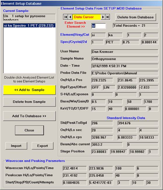
Scroll through the list of elements (records) and find the desired element and setup using the data cursor. Use the left, right arrows (top, center) to move through the database. To see all the setups for a particular element, enter the element symbol into the Search Element text field and use the arrow keys as before. To see all element setups again, simply clear the Search Element text field. To view the most recent addition(s) to the SETUP database, click the  button on the data cursor.
Here, the user browses through the records and selects the appropriate silicon (si) entry as the first element setup to load. The output list order of elements will follow this list.
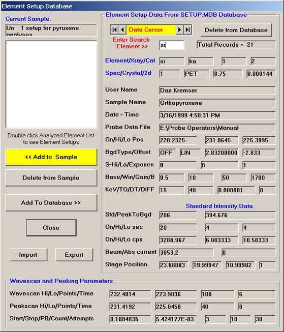
Click the << Add to Sample button to add the element setup to the current sample.
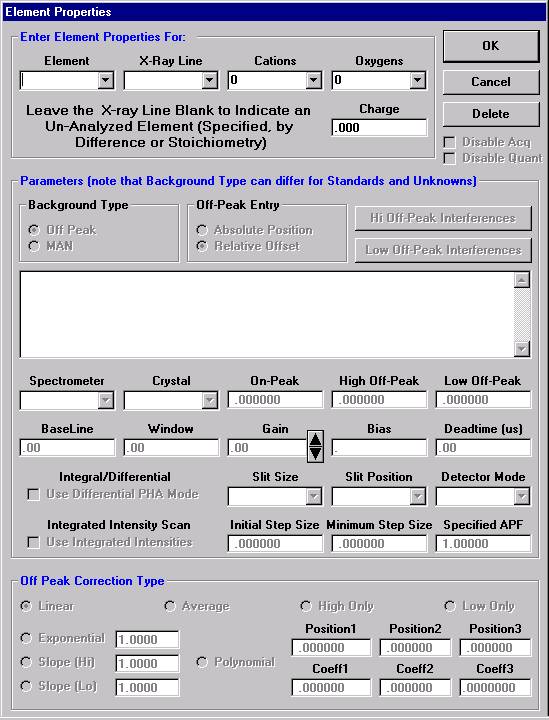
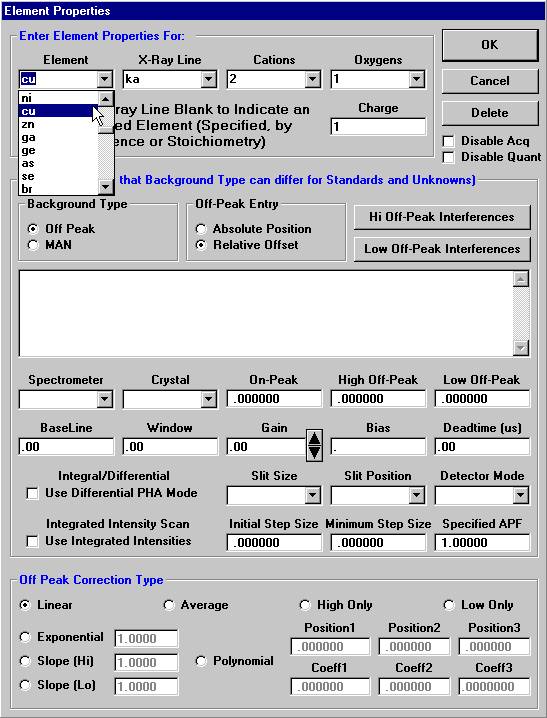
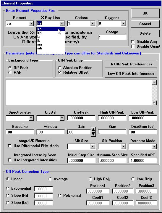
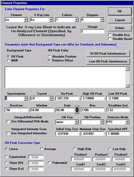
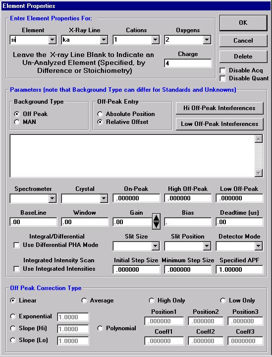
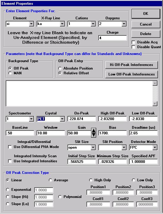
The Element Properties window for silicon appears.
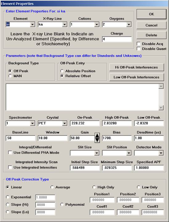
Edit if required, then click the OK button to accept
these values.
The silicon record is then listed in the text field under the previously defined sample name.
Continue browsing the element setup database and add all required element setups desired to the sample.
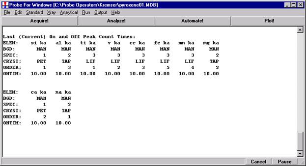
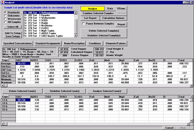
A typical pyroxene element setup list is shown below.
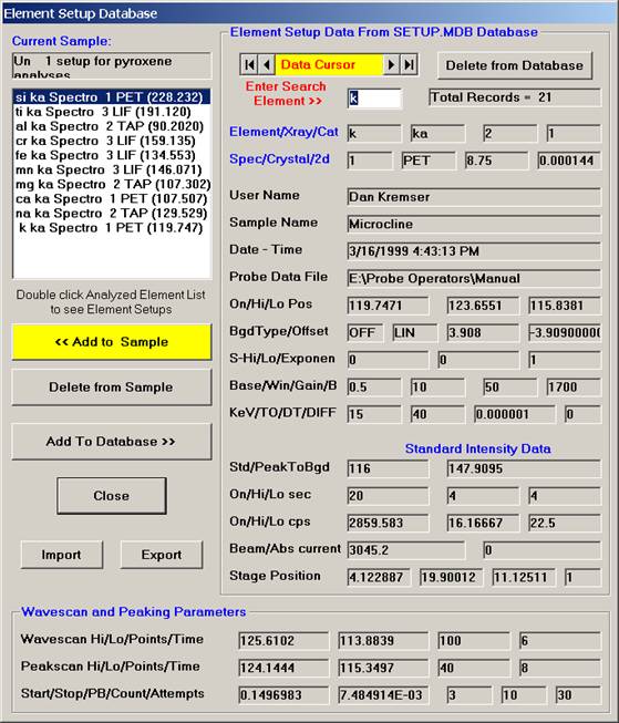
Click the Close button when finished. The New Sample window reappears.
Click the OK button, returning to the Acquire! window. Don’t forget to add oxygen as a specified element to the list for stoichiometry and other calculations. Note specified elements cannot be saved to the SETUP.MDB database.
Normally, Probe for EPMA uses the sample setup from the last unknown (or standard if there are no unknown samples) to create the next new sample setup. Sample setups on the other hand are designed to allow the user to easily recall a previous sample setup within a current run. This allows the user to create and re-use multiple setups comprised of different groups of elements within a single run. In the example below, sample setups for pyroxene and olivine will be created, each with a different set of elements and conditions, that may be recalled at anytime during the current probe run.
The saving of a sample setup actually saves only a pointer to the sample selected. All of this sample’s acquisition and calculation options, elements/cations, standard assignments, etc will be utilized when a new sample is created based on this sample setup. However, because counting time and the associated unknown count factor is treated by Probe for EPMA as data as opposed to setup information, it is necessary (if the user wants this information to be carried over) to acquire at least one data point with the sample setup prior to saving it as a sample setup.
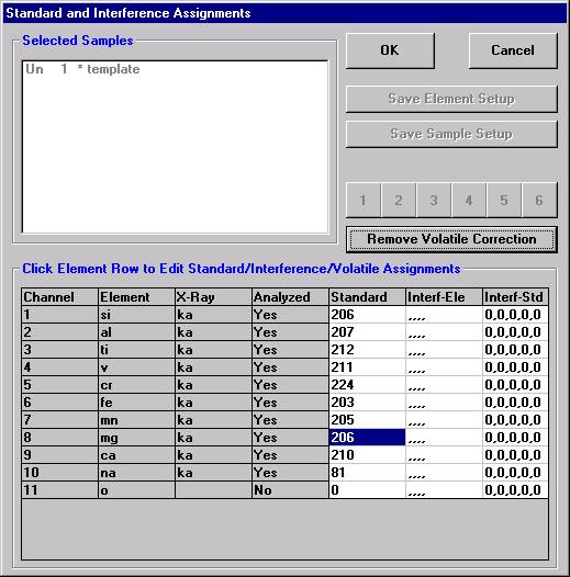
A new Probe for EPMA run is opened in the usual manner. Ten elements and appropriate standards for pyroxenes are loaded from the SETUP.MDB database and the STANDARD.MDB database, respectively. Each element is then calibrated and standardized. Count times, acquisition and calculation options are adjusted to optimize the analyses and output requirements. And finally, a pyroxene standard is run once to update count time information.
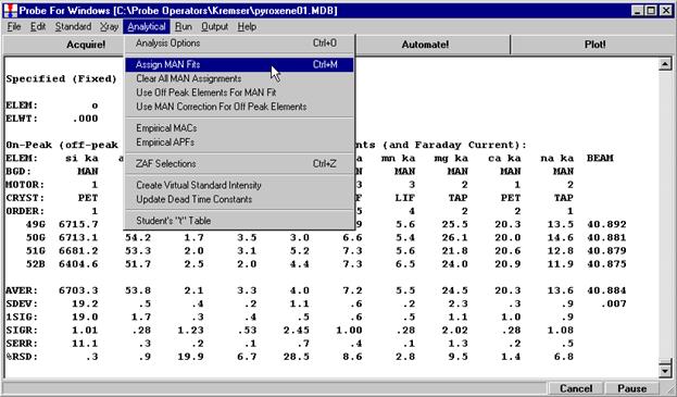
To save the just calibrated pyroxene sample as a sample setup, start by clicking the Elements/Cations button from the Analyze! window.
The Analyzed and Specified Elements dialog box appears.
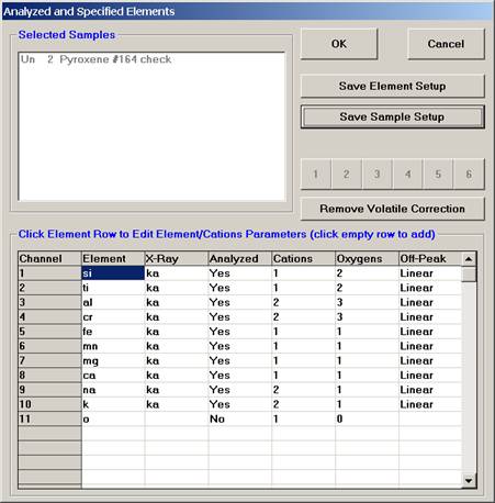
Click the Save Sample Setup button.
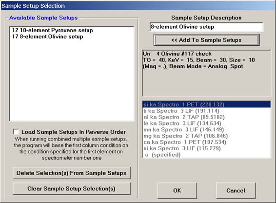
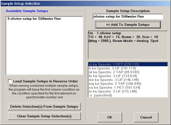
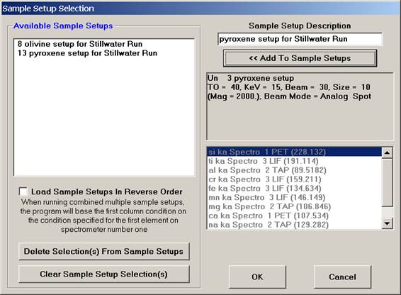
The Sample Setup Selection window opens.
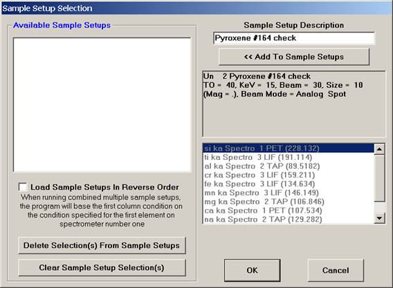
Edit the Sample Setup Description text box as desired.
Click the << Add To Sample Setups button.
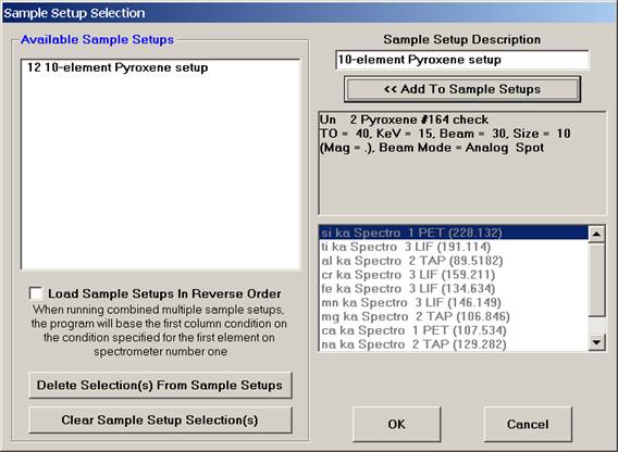
The Sample Setup Selection window appears as below. Note: the first number (12) represents the sample’s row number and can be seen listed using the Run | List Sample Names menu.
Click the OK button, returning to the Analyzed and Specified Elements window.
Click the OK button of the Analyzed and Specified Elements window returning to the Analyze! window.
Return to the Acquire! window to create a new sample.

Click the New Sample button.
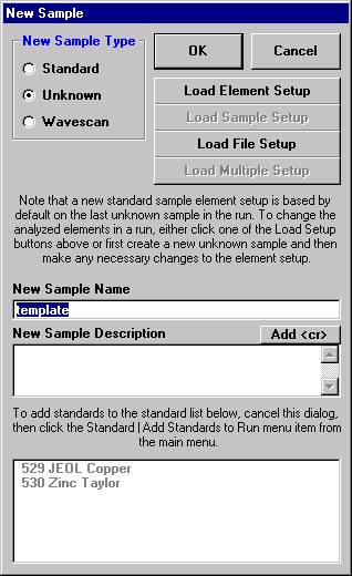
Edit the New Sample Name text field. Here, the user will establish an olivine sample setup.
Several paths may be taken from here to load new elements for the olivine sample. To enter an entirely new list of elements and parameters it might be easier to click the OK button and follow the Element/Cations button of the Acquire! window to the Element Properties dialog.
If (as in this example) only minor changes to a sample are required then from the New Sample window, click the Load Element Setup button.
The Element Setup Database opens.
Edit the previous pyroxene list, in this example chromium, sodium, potassium are eliminated from the list by highlighting each element and clicking the Delete from Sample button. If additional elements are required, recall them at this time (nickel is added in this example).
After editing, the window appears as below.
Click the Close button of the Element Setup Database, returning to the New Sample window.
Click the OK button in the New Sample window, returning to the Acquire! window.
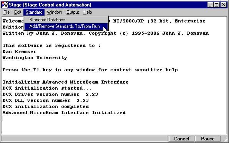
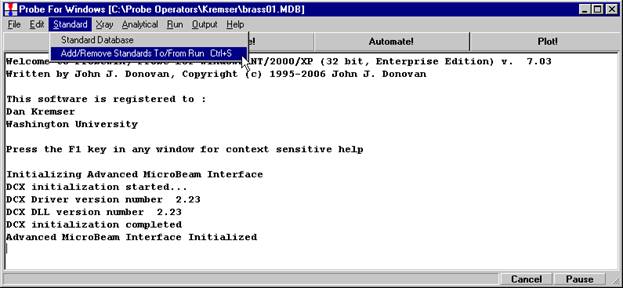
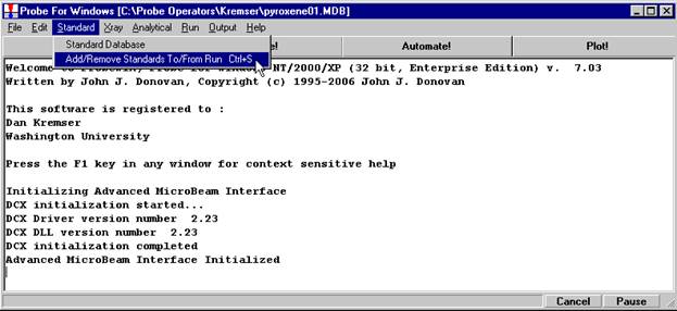
If different standard choices are required they should be added from the STANDARD.MDB database at this point. Use the Standard | Add/Remove Standards To/From Run menu in the main Probe for EPMA log window.
Recalibrate and standardize all new elements and adjust count times, acquisition, and calculation options to optimize for olivine analysis. Run an olivine standard to obtain data and check the calibration.
From the Analyze! window, click the Elements/Cations button.
The Analyzed and Specified Elements window opens, click the Save Sample Setup button.
The Sample Setup Selection window appears. Edit the Sample Setup Description text field and click the << Add To Sample Setups button, storing the Olivine setup along with the previously stored Pyroxene setup.
Click the OK button returning to the Analyzed and Specified Elements window.
Click the OK button to go back to the Analyze! window.
Any number of sample setups can be created as described above.
The user now has two calibrated sample setups available to analyze any pyroxene or olivine in the samples supplied for microprobe analysis. The olivine setup (last) is currently active however to recall any other sample setup, follow the steps outlined below.
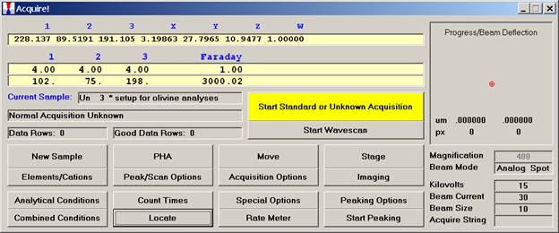
Bring forward the Acquire! window. Move to the next unknown analysis spot, in this example the user wishes to analyze several pyroxene grains.
Click the New Sample button.
The New Sample window opens. Enter the appropriate text into the New Sample Name and New Sample Description fields.
Click the Load Sample Setup button.
This opens the Sample Setup Selection window.
Select the Pyroxene setup, highlighting it allows the operator to view the element list.
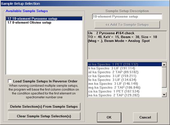
Click the OK button of the Sample Setup Selection window to load the sample setup.
The program returns to the New Sample window. Click the OK button.
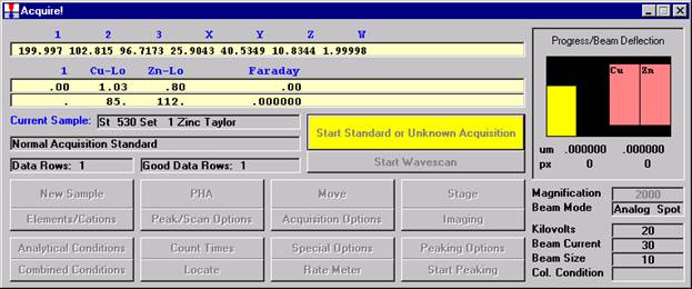
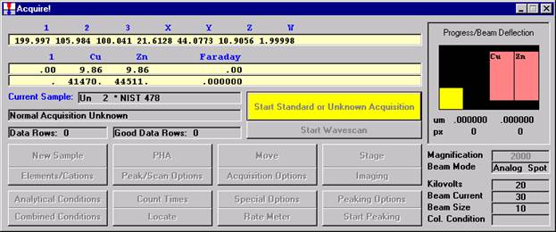
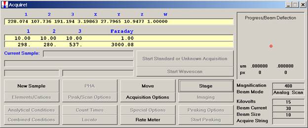
The Acquire! window reappears.

Double check your spot selection and focus and click the Start Standard or Unknown Acquisition button to initiate data acquisition.
The availability of multiple sample setups during the course of automated unknown analysis gives the user tremendous flexibility. Upon activation of the Use Digitized Sample Setups button in the Automate! window, each unknown analysis may be based on a different sample setup that was specified when the unknown sample position was digitized. See the User’s Guide and Reference documentation for more details.
To load any sample setup from a previous probe run file, the file setup option is provided. These file setups are old Probe database files that contain old sample setups and may or may not contain standardization count intensity data.
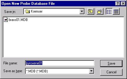
The example below will illustrate how to use the file setup option to easily import two different (an olivine and a pyroxene) sample setups into the current new probe run. Open a new Probe for EPMA run and click the New Sample button from the Acquire! window.
The New Sample window appears. Edit the New Sample Name text box.

Click the Load File Setup button.
The Load File Setup window opens and will list all available Probe for EPMA files that can be loaded. The initial available Probe Run Files directory pointer is the location specified when opening a new probe database file earlier. Move to another directory location if necessary. The last file listed in the available Probe Run Files along with the last entry in the Samples List will be shown by default.
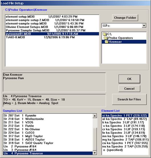
In this example, the file STILLWATER PY-OL RUN1.MDB was newly created and the user will load both an olivine and a pyroxene sample setup into this file.
Scroll through the available Probe Run Files list and highlight the file to load from. The last sample setup will be displayed in the Samples List and Element List text field. Next, select the sample setup that you wish to load into the new probe run. All of the run parameters and options for that sample setup will be loaded. The only parameters not loaded are the nominal beam current and the volatile element assignments since they are unknown sample specific.
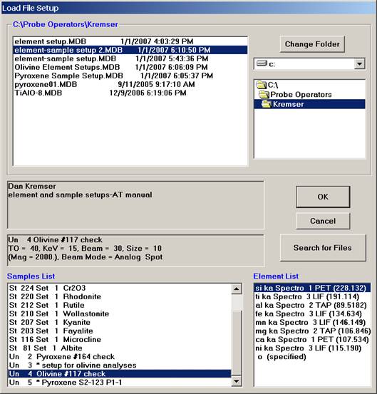
Click the OK button to load in this sample setup of interest.
The NewFileSetupLoadStandardData window appears next, asking whether the user wants the previous standard intensity data to be loaded as well.
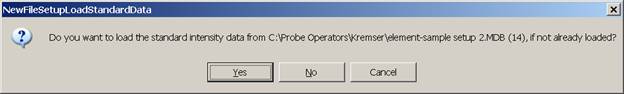
Selecting Yes would load the old standard intensity data from the file setup into this new run. Depending on the stability of your instrument, it may or may not be necessary to re-standardize some or all of the standards. In this case, the user chooses to load the standard intensity data, selecting the Yes button.
The NewFileSetupLoadStandardData window appears.
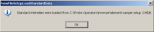
Click the OK button.
The New Sample dialog box reappears.
Click the OK button to complete the loading of the olivine sample setup from the old probe run.
The program now returns to the fully active Acquire! window.
The user then opens the Analyze! window to save this olivine setup as a sample setup in this current probe run.
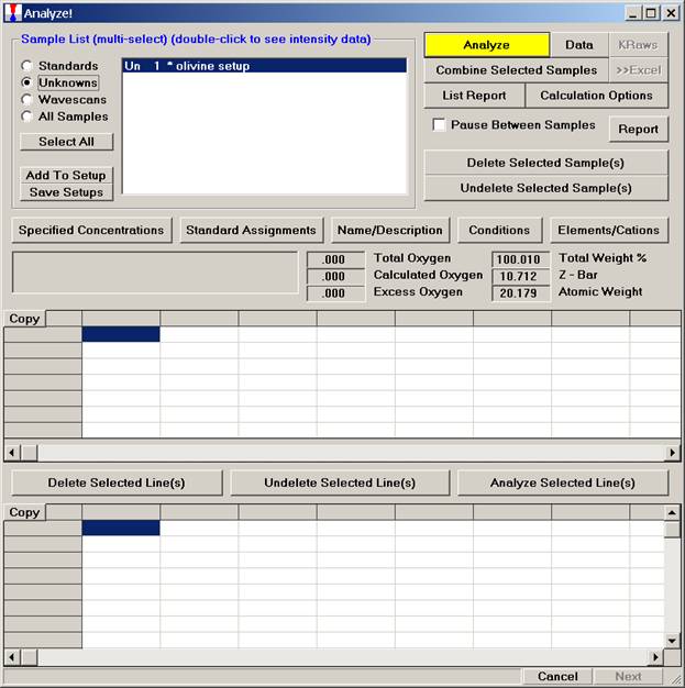
Click the Elements/Cations button, opening the Analyzed and Specified Elements window.
Click the Save Sample Setups button.
The Sample Setup Selection window opens. Edit the Sample Setup Description text box and click the << Add To Sample Setups button, resulting in the following window.
Click the OK button, returning to the Analyzed and Specified Elements window. Click this OK button to return to the Analyze! window.
If another, previously created sample setup is needed for this current probe run, open the New Sample window and follow the
instructions of the past eight pages.
Remember to save each sample setup in the Sample Setup Selection window as described above.
Returning to the Acquire! window, the user can now employ either sample setup for probe work.

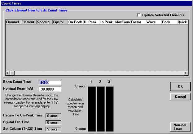
This feature is useful if an EDS detector is not available or WDS resolution over the entire spectrometer range is required. The program will move each spectrometer currently assigned to it’s upper limit and then continuously scan each spectrometer to it’s lower travel limit while acquiring simultaneous count data. The count time used for the Quick Wavescan Acquisition is specified in the Count Times dialog box, opened from the Acquire! window. The current sample setup specifies which spectrometer and reflecting crystal to use. The program uses the spectrometer calibration of the first acquired element (order = 1) in the sample.
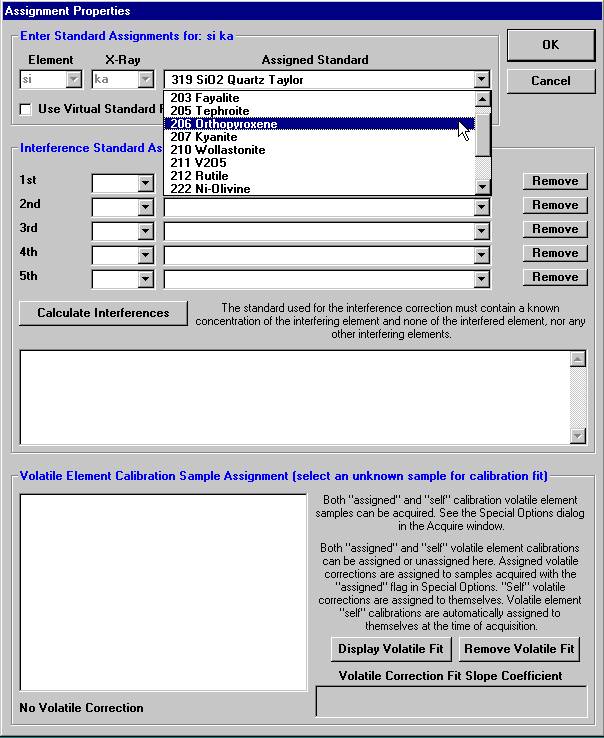
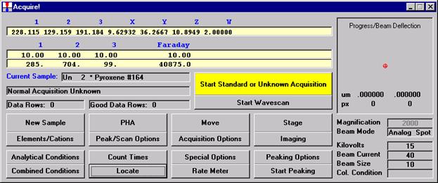
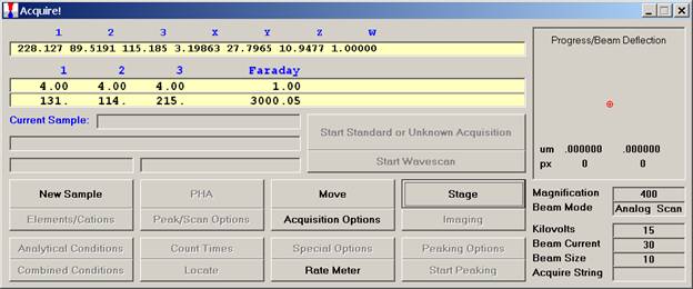
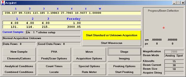
From an open Probe for EPMA run, containing an unknown sample and the appropriate unknown under the crosshairs, click the Special Options button from the Acquire! window.

This opens the Volatile Calibration and Quick Wavescan Samples window. Note the default acquisition option is Normal Acquisition.
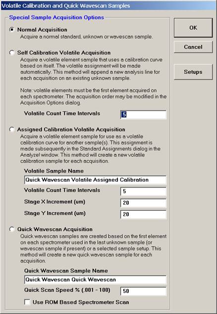
Select the Quick Wavescan Acquisition dialog button. Enter a Quick Wavescan Sample Name and Quick Scan Speed into the text fields. The smaller the scan speed percentage the slower the spectrometer will travel per second and of course each instrument would require different settings.
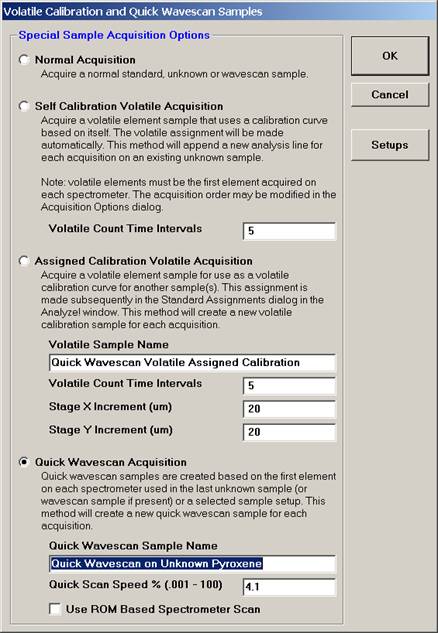
Click the OK button to return to the Acquire! window.
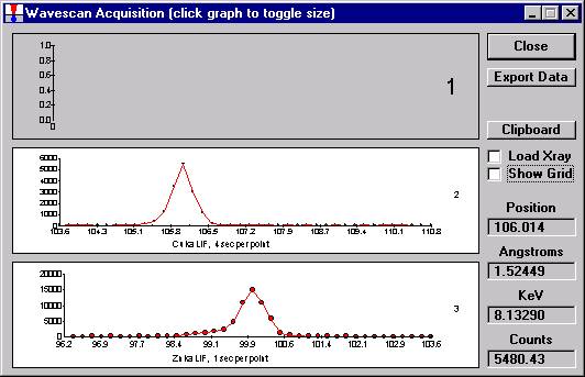
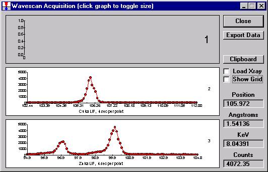
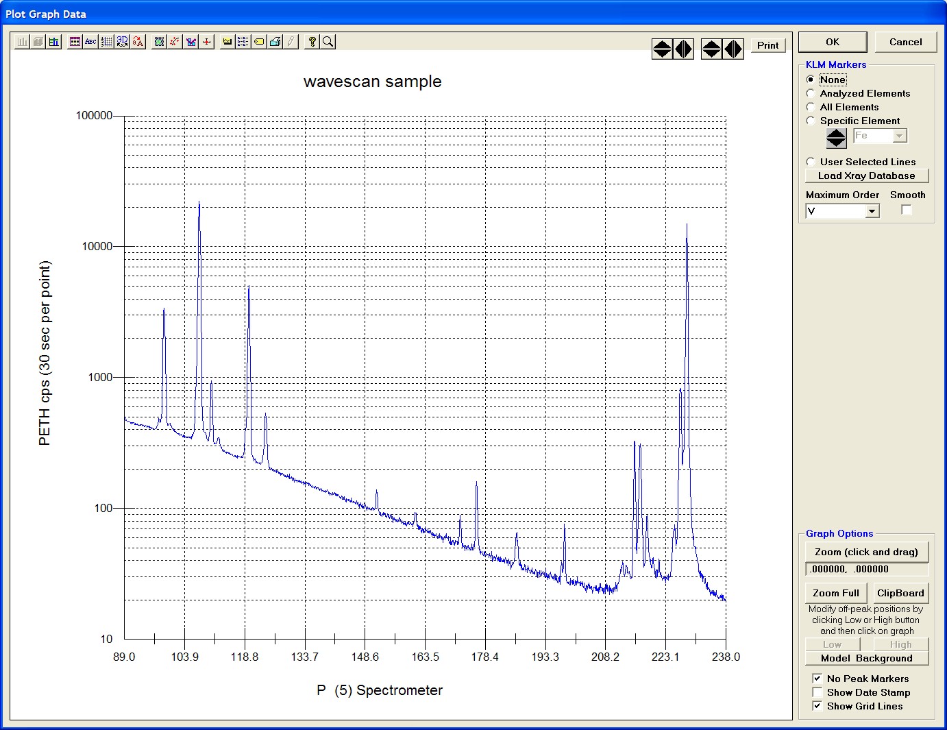
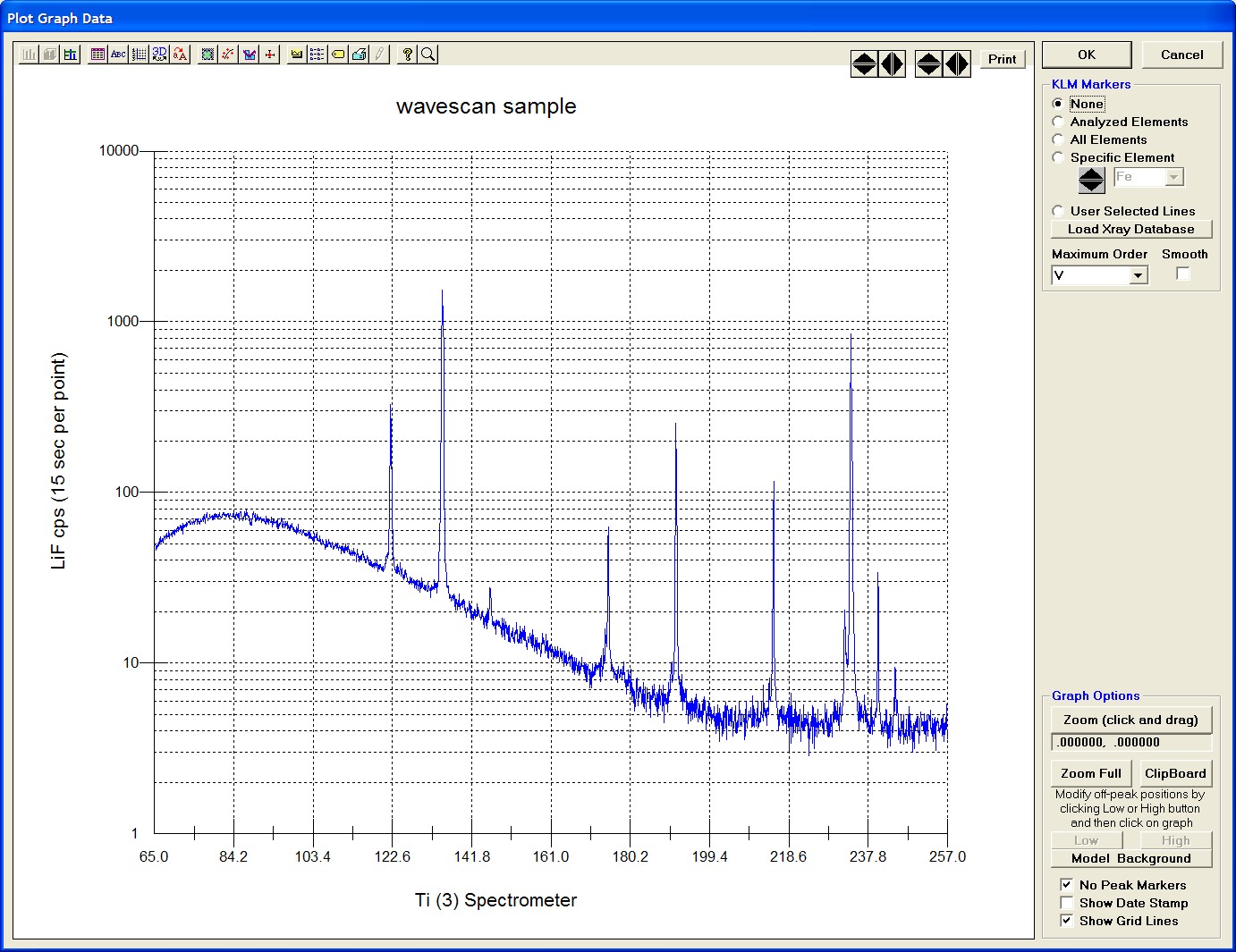
To initiate the quick wavescan acquisition, click the Start Wavescan button in the Acquire! window. A new wavescan sample is automatically started using the sample name just supplied. The spectrometers move to their respective upper limits and proceed with the wavescan. The Wavescan Acquisition window opens and real time data display is viewable. A completed three-spectrometer Wavescan Acquisition window appears below.
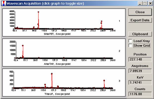
The size of each graph maybe expanded (as shown below) by clicking on the relevant wavescan.
Upon completion of the quick wavescan, the data may be exported via the Export Data button to an ASCII file or examined in more detail along with KLM marker overlay capabilities from the Plot! window. Printing of the quick wavescan is possible by selecting the Print option under the Graph Data window (see next section for a specific example).
Another unique feature of Probe for EPMA is the ability to acquire calibrated multi-element wavescans. This provides an easy and rapid method to scan all elements in a sample for off-peak interferences. The example below will illustrate calibrated wavescans on a ten-element pyroxene sample and the adjustment of off-peak background positions.
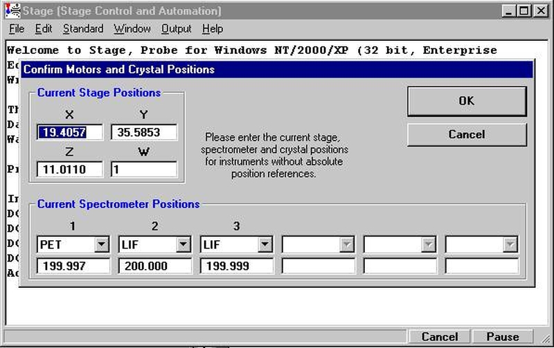
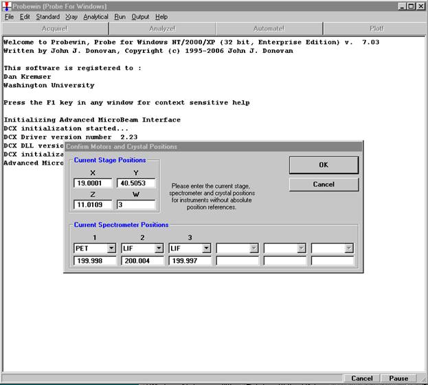
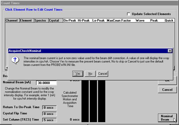
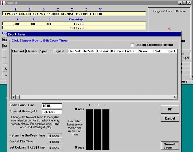
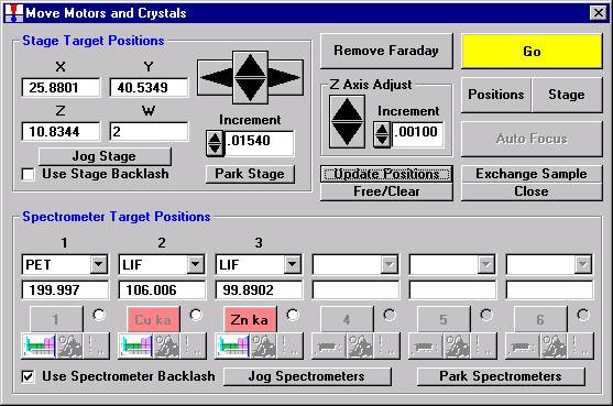
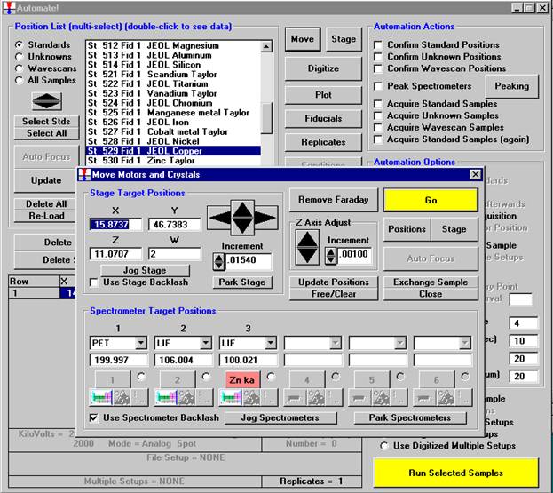
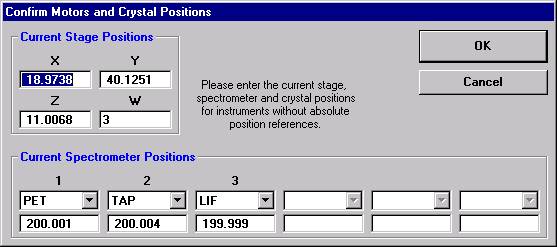
Open a new Probe for EPMA run in the usual manner. Confirm motor and crystal positions in the Move Motors and Crystals window. Click the Acquire! button and allow the program to acquire a nominal beam current (in a new run). Click the New Sample button and create a sample using the elements of interest. Next, re-peak the elements using either manual or automatic peaking on the appropriate standards. This calibrates the spectrometer motors. And finally, move to the sample to perform
the calibrated wavescan.
From the Acquire! window, click the New Sample button to create a wavescan sample.
The New Sample window opens. Select the Wavescan check button as the New Sample Type. Edit the New Sample Name and New Sample Description text fields.
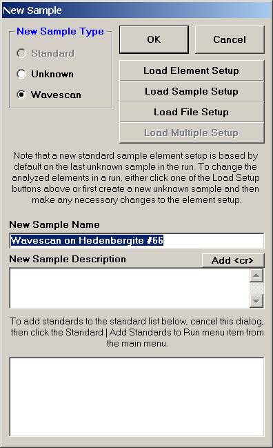
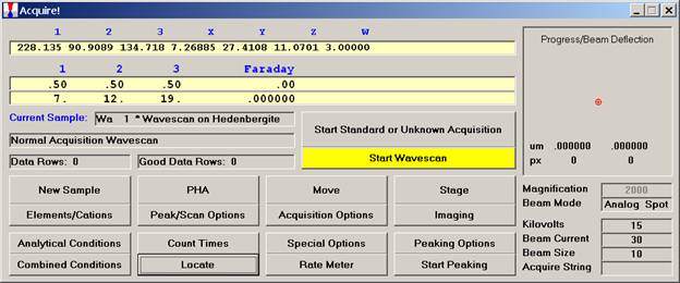
Click the OK button.
The program returns to the Acquire! window.
To modify the wavescan range and/or number of data points to be collected, click on the Peak/Scan Options button in the Acquire! window.
Select the Wave Scan Limits check button under Display: and click on the appropriate element row to edit the parameters. The stage may also be moved (incremented) during the acquisition using the Stage Step During Peakscan/Wavescan or Peaking (X and Y Axis) check box and Increment Size (microns) text field.
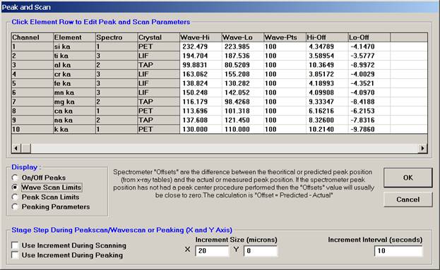
The user wishes to adjust the spectrometer start and stop values for k ka, click on the row of that element.
This opens the Peak and Scan Properties window. Adjust the appropriate values.
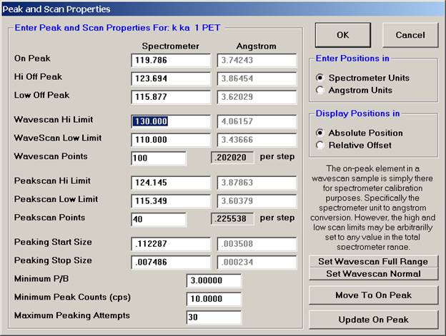
Click the OK button of the Peak and Scan Properties window when done editing.
Then click the OK of Peak and Scan Properties to close.
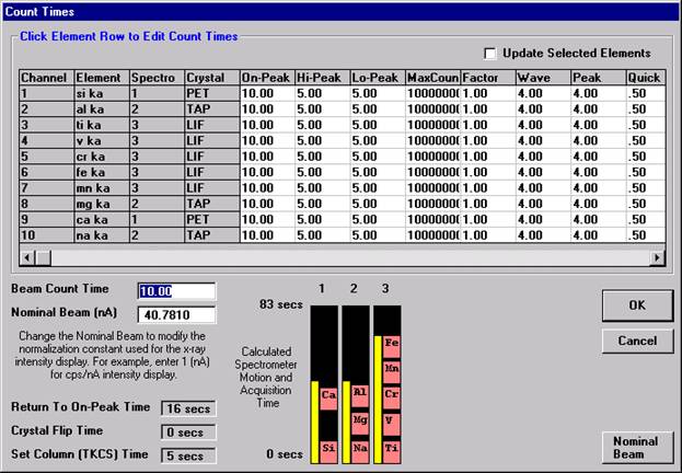
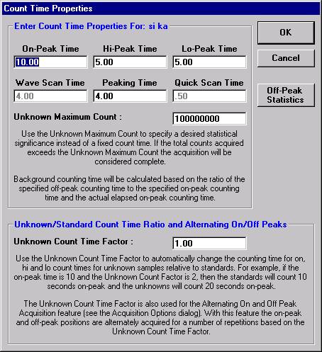
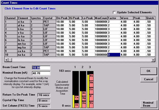
Wavescan count times for each element are adjusted via the Count Times button in the Acquire! window.
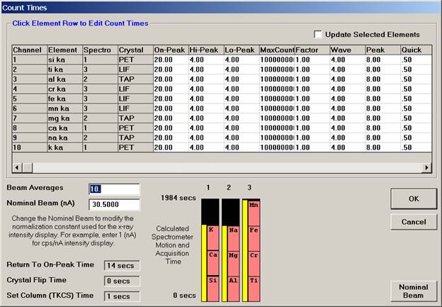
Click on the appropriate element row to edit the wavescan time. Edit the Count Time Properties dialog box and then click it’s OK button to close.
Click the OK button to close the Count Times window.
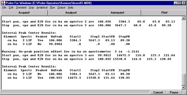
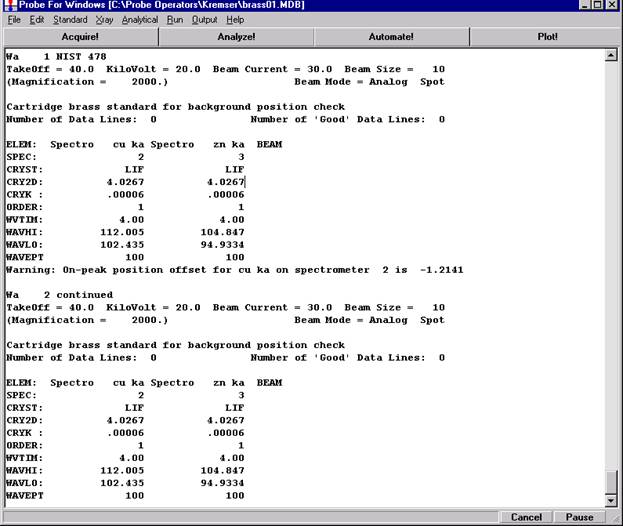
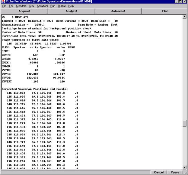
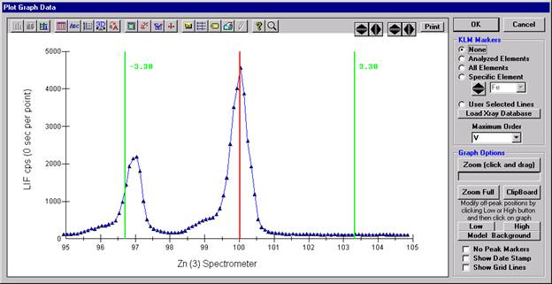
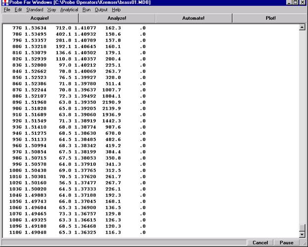
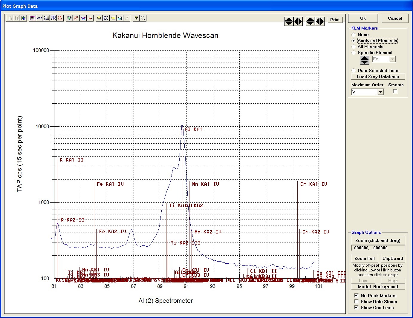
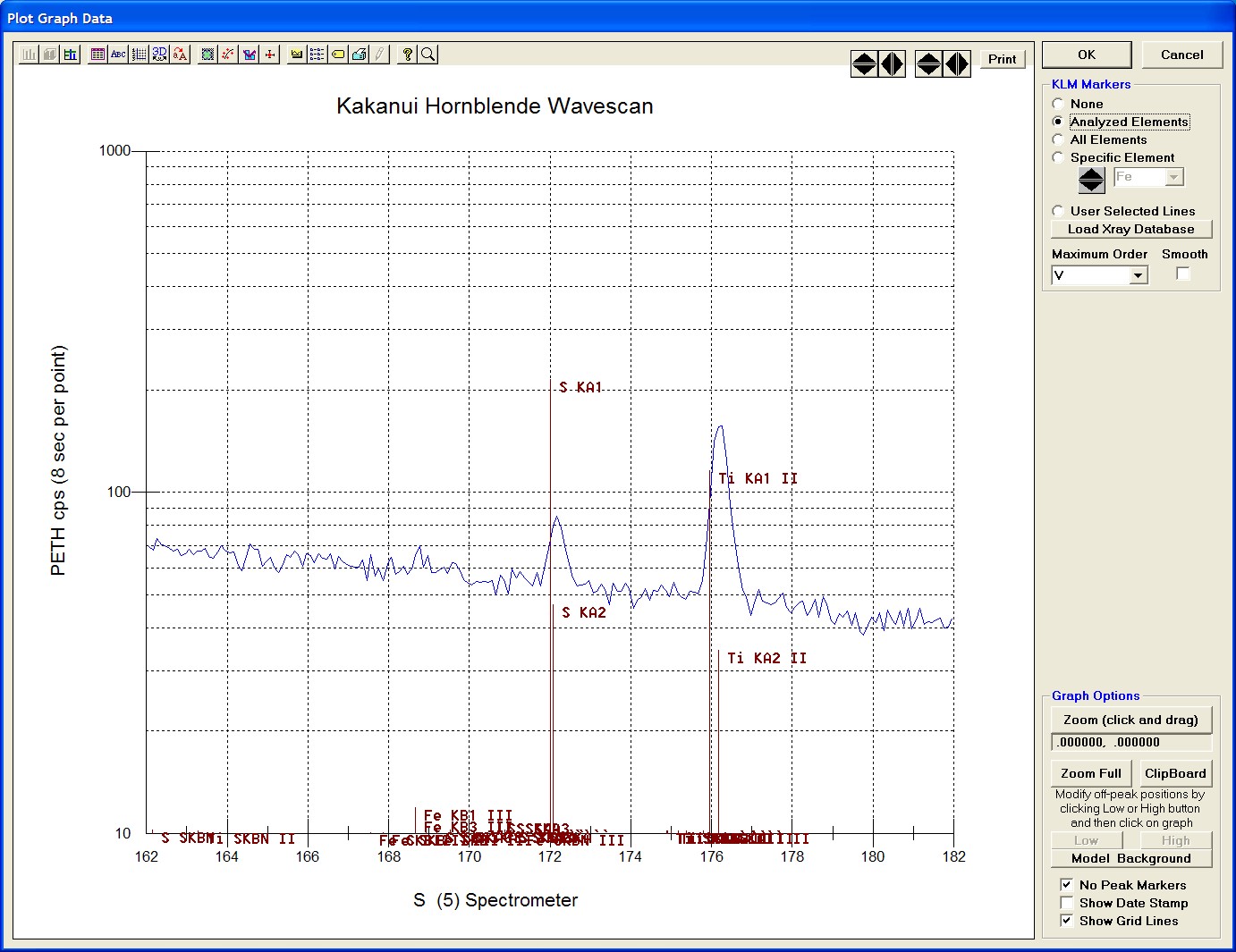
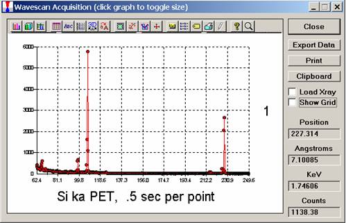
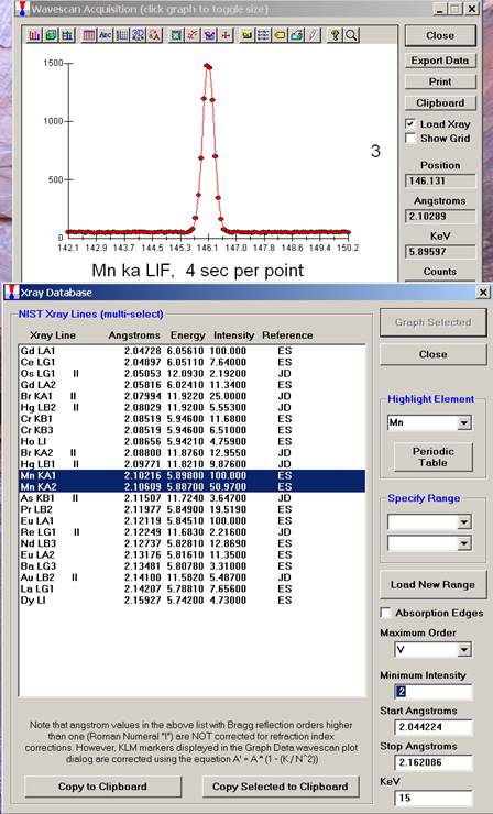
Click the Start Wavescan button in the Acquire! window to initiate the calibrated multi-element wavescan. The Wavescan Acquisition window opens. The program will automatically start acquiring the wavescan ranges selected. If more than one element is assigned to a given spectrometer, the program will automatically go to the next element’s wavescan range after the previous wavescan element range is completed. The order of acquisition is defined in the Acquisition Options window. Below illustrates a completed wavescan acquisition.
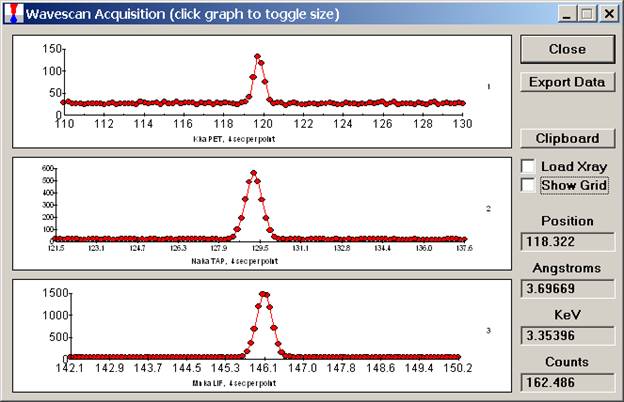
As the wavescan is acquiring data, the wavescan graph may be viewed in greater detail by clicking on the graph to toggle/expand the display size.
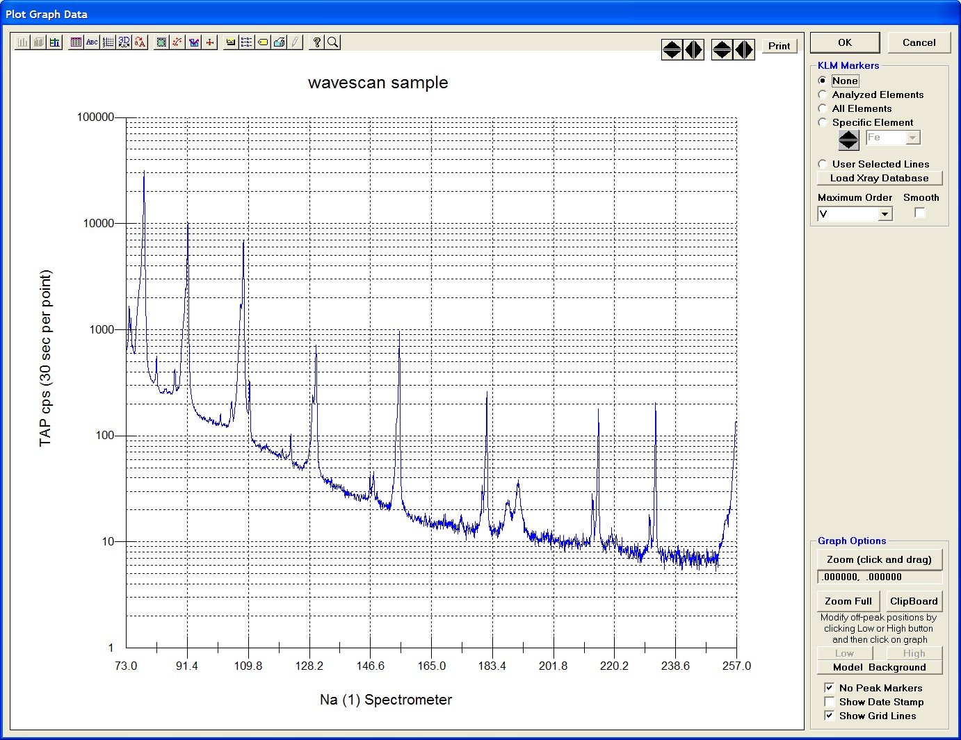
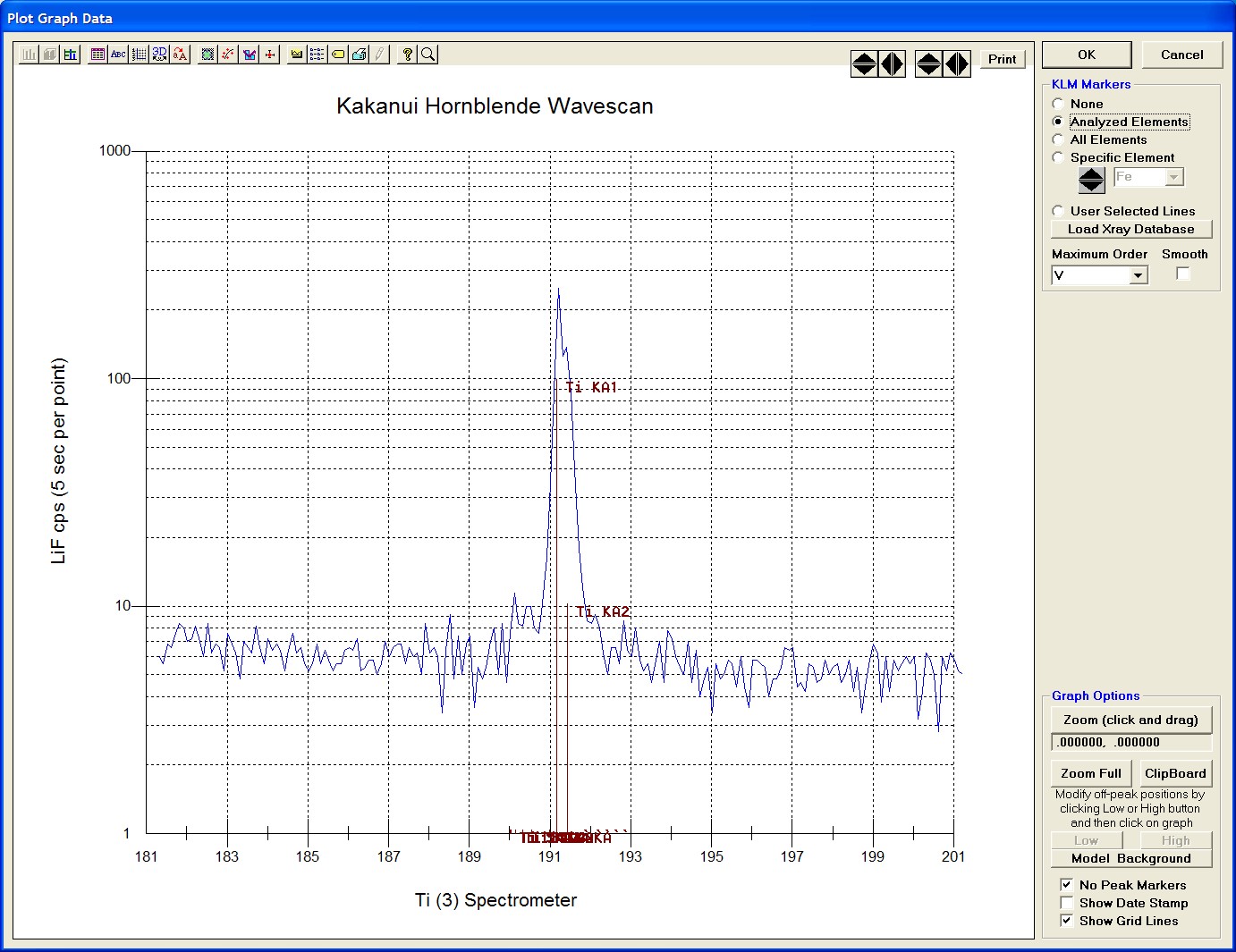
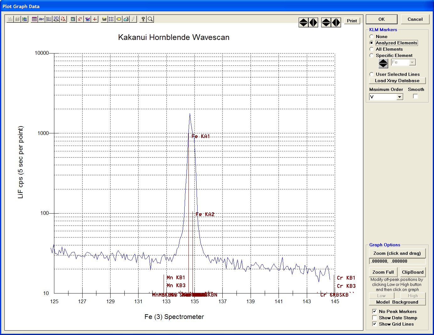
The top portion of the following screen capture illustrates an expanded view of the manganese x-ray wavescan on spectrometer 3.
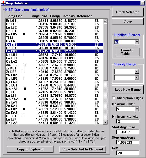
The Position (spectrometer units), Angstroms, and Counts in any channel may be read by placing the cursor on the graph. Selecting the Load Xray check box and clicking the graph, loads the NIST x-ray database (also seen below). The location of the manganese K alpha x-ray lines are highlighted.
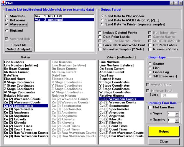
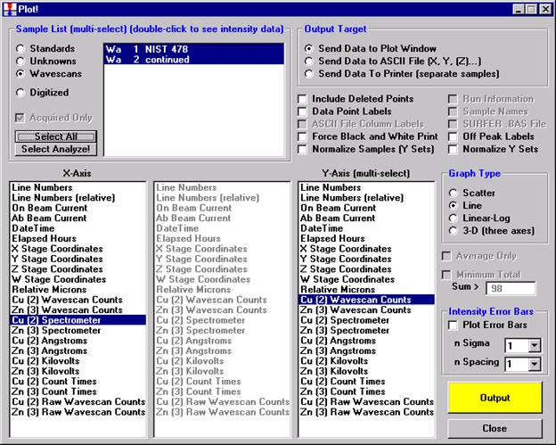
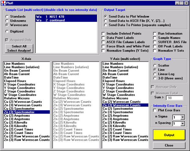
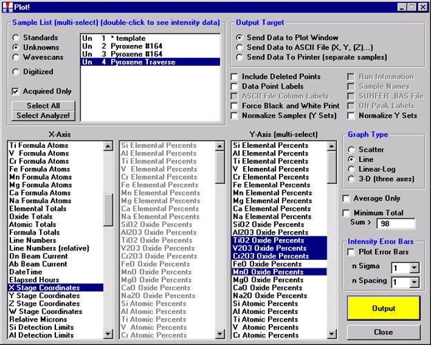
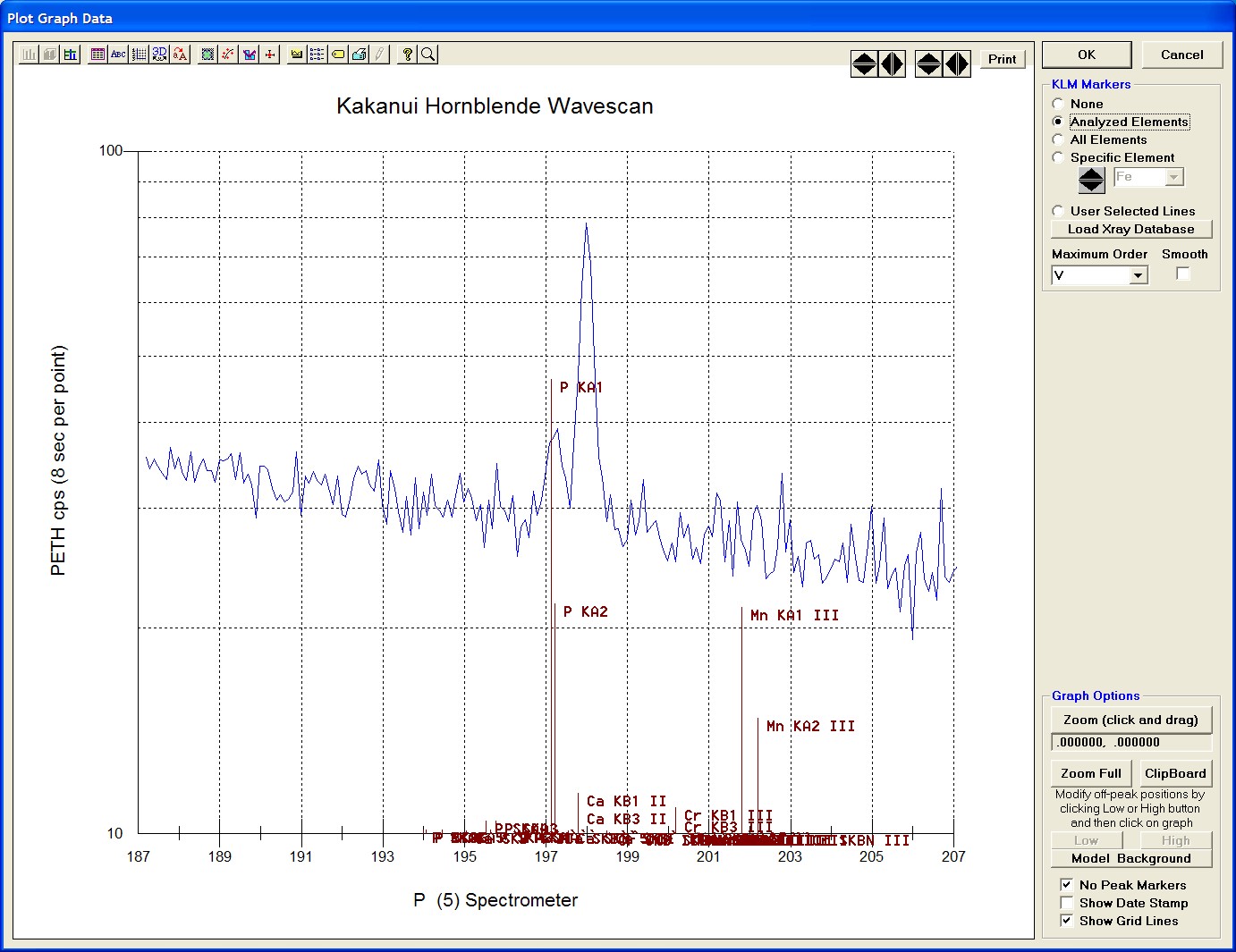
After all wavescans have been acquired on the sample, the user would typically inspect off-peak interferences and background locations by using the Plot! window. Note that if more than 50 points were acquired in a wavescan be sure to highlight all of the “continued” samples associated with the wavescan.
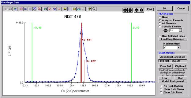
Select an X-Axis parameter (normally a specific spectrometer) and a Y-Axis parameter (normally the associated wavescan counts). The number (X) after the element in each List designates the spectrometer employed to collect the data. Finally, click the Line check button under Graph Type.
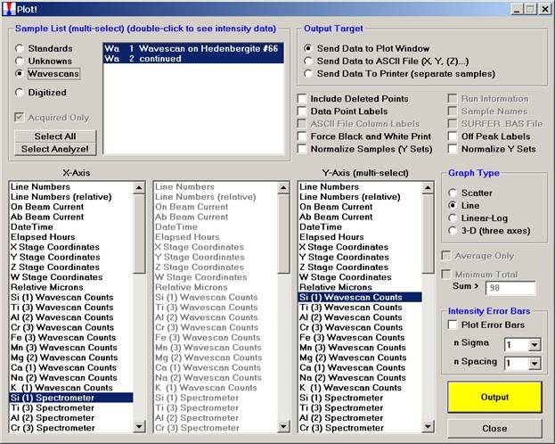
Click the Output button to graph the wavescan.
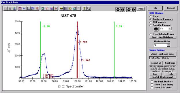
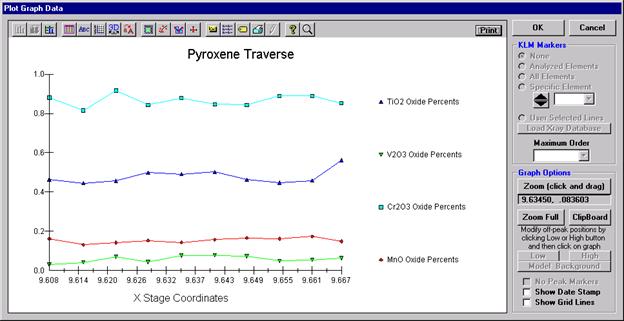
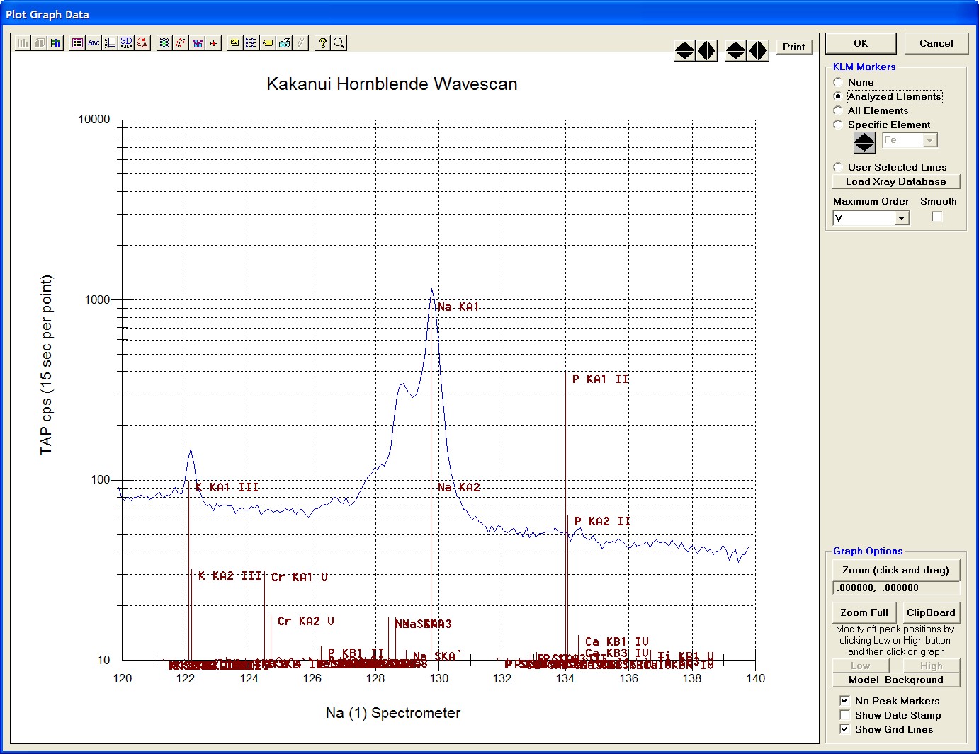
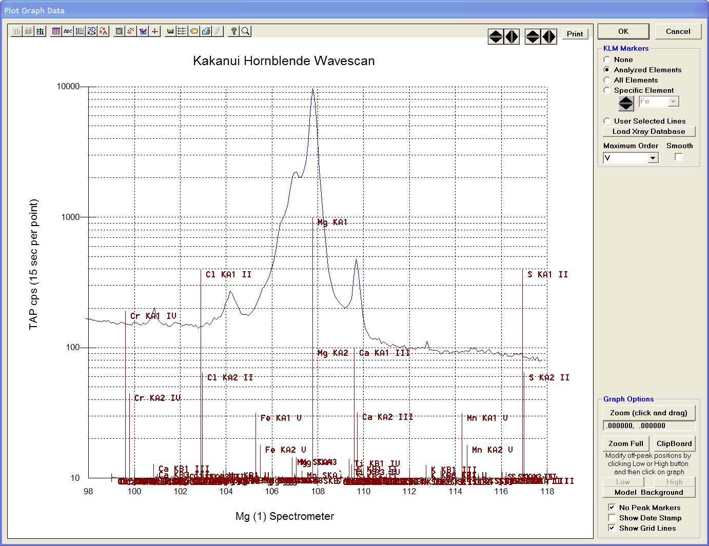
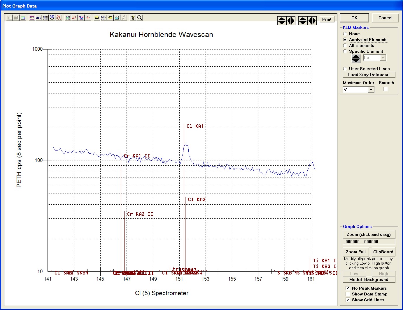
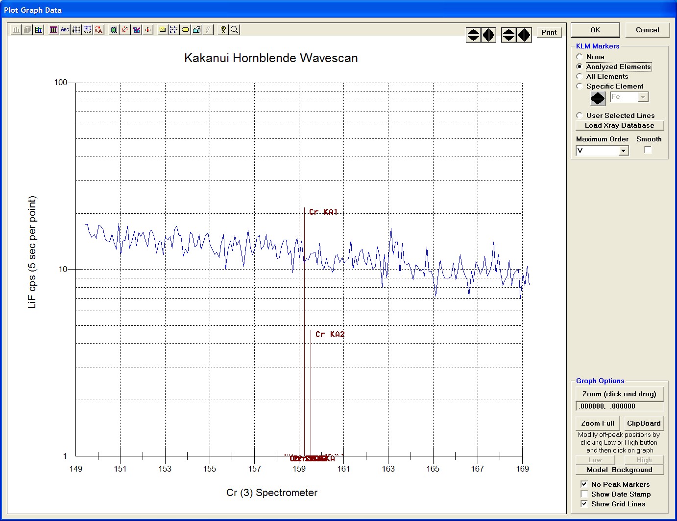
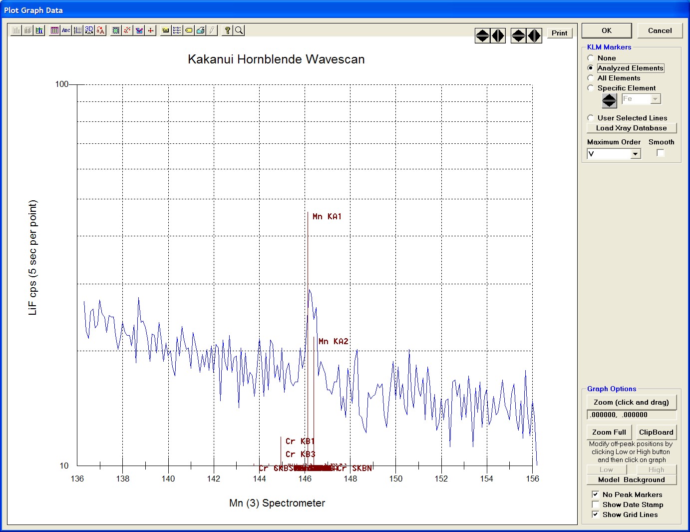
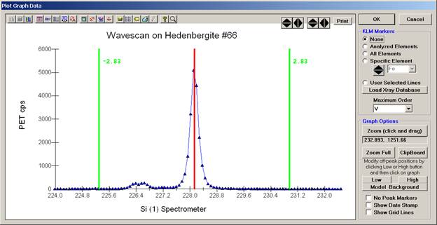
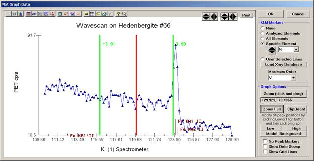
The Graph Data window opens displaying the plotted components. The currently selected off-peak positions for background measurements are also indicated (green).
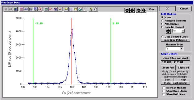
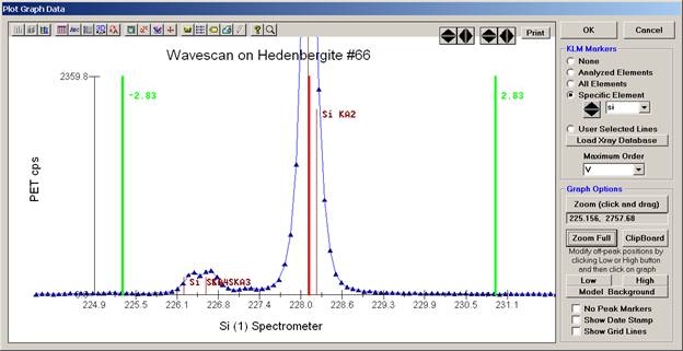
To evaluate potential interferences select a KLM Markers option (Analyzed Elements check button, for instance) to view the KLM markers or use the Load Xray Database button.
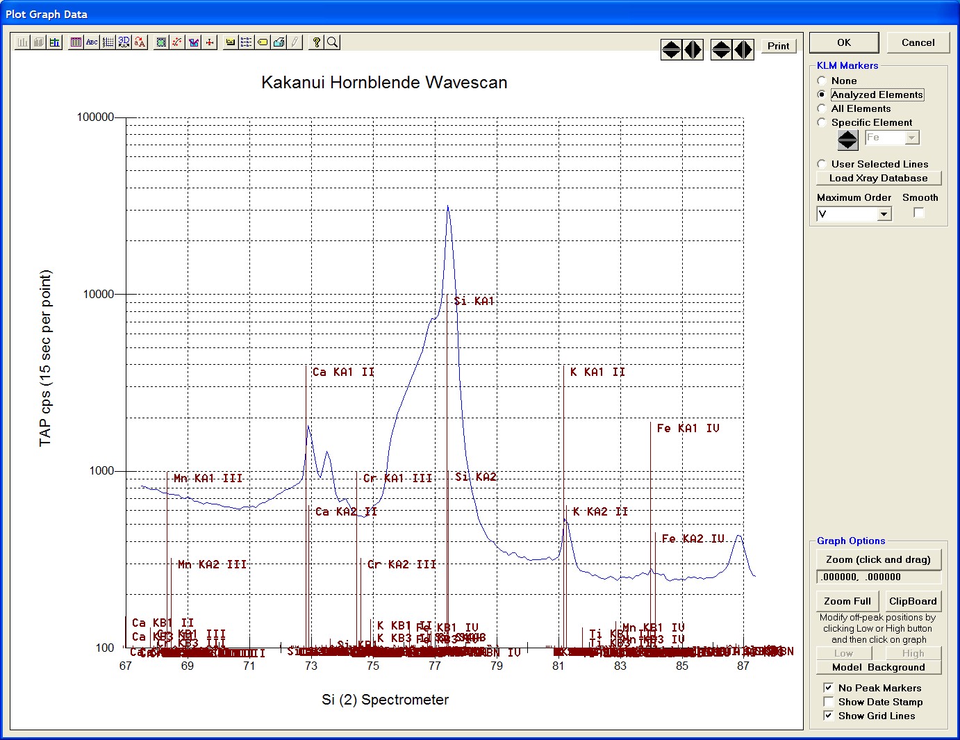
Click and drag the mouse to Zoom in on any portion of the graph. The Graph Data window open below illustrates this powerful feature and the identification of the small x-ray peaks (satellite lines) to the high-energy side of the main silicon x-ray peak.
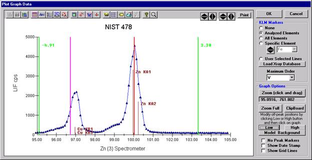
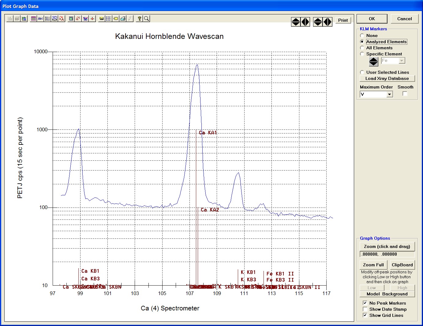
The off-peak positions for background determinations for quantitative samples are adjusted with the Low and High buttons (located lower right of Graph Data window).
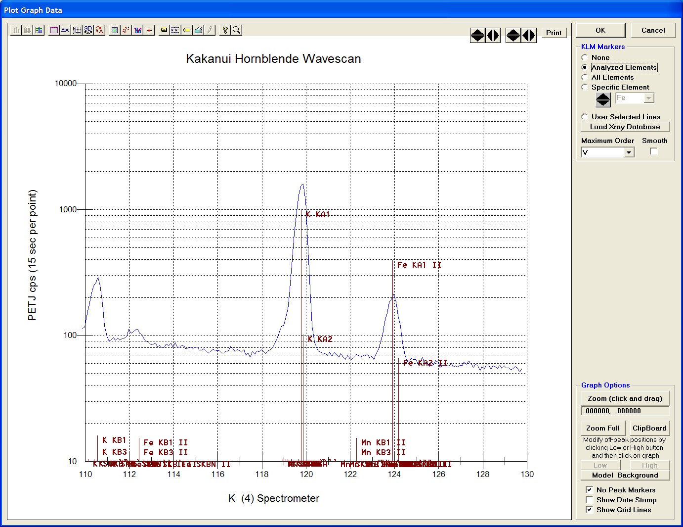
In the next screen capture, detailing K (1) Wavescan Counts (PET cps) versus K (1) Spectrometer, the user will note that the high background position falls on top of the signal from Fe Kα1,2 second order. This could give an anonymously high background reading on this sample, if iron is present. Therefore, the user chooses to move the high background slightly to a lower spectrometer position.
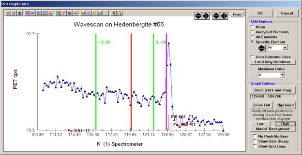
Click the High button, move the mouse cursor (note it appears as a cross on the graph) to an appropriate new position and click the graph.
The graph will update the new off-peak position (purple is the old position, green the new position).
Click the OK button of the Graph Data window. The GetPeakSave window appears.
Click the OK button to accept and store the new high background position for K Kα x-rays.
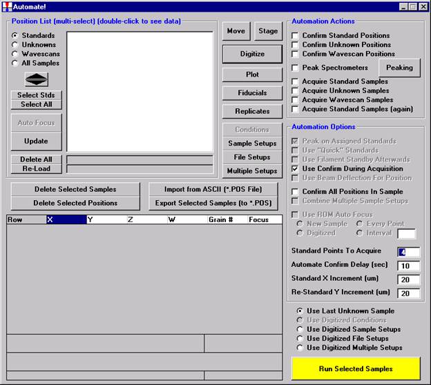
Another useful feature of Probe for EPMA is the ability to perform automated polygon gridded analyses of unknowns. After acquiring the digitized data set, Probe for EPMA can create a script file (if the SURFER.BAS file option is selected in the Plot! window) for use with SURFER for Windows to automatically generate contour, surface and *.GRD concentration files of your data. These *.GRD files can be imported into MicroImage for viewing in false color. The images will be quantitatively registered during the import process so that color represents elemental or oxide concentration.
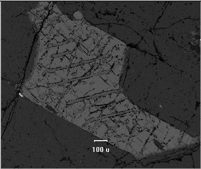
In this example an unknown and complexly exsolved pyroxene (see image below) will be gridded and digitized, then run quantitatively. Move to the unknown grain location.
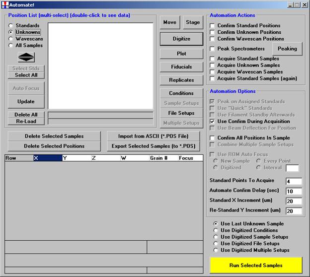
Click the Digitize button of the Automate! window.
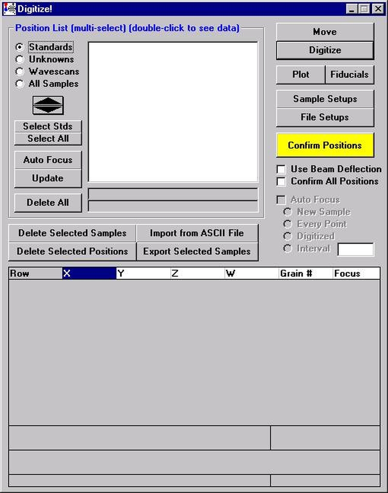
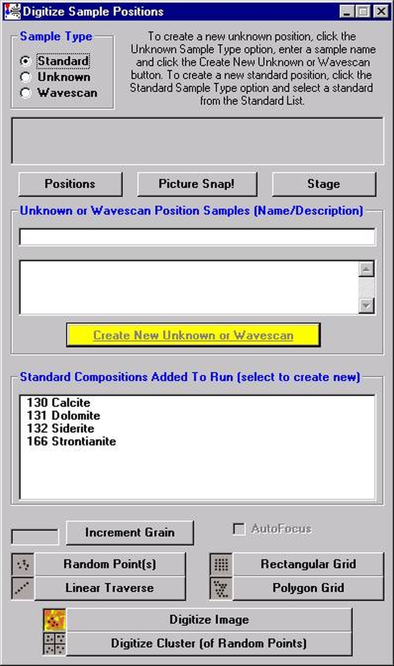
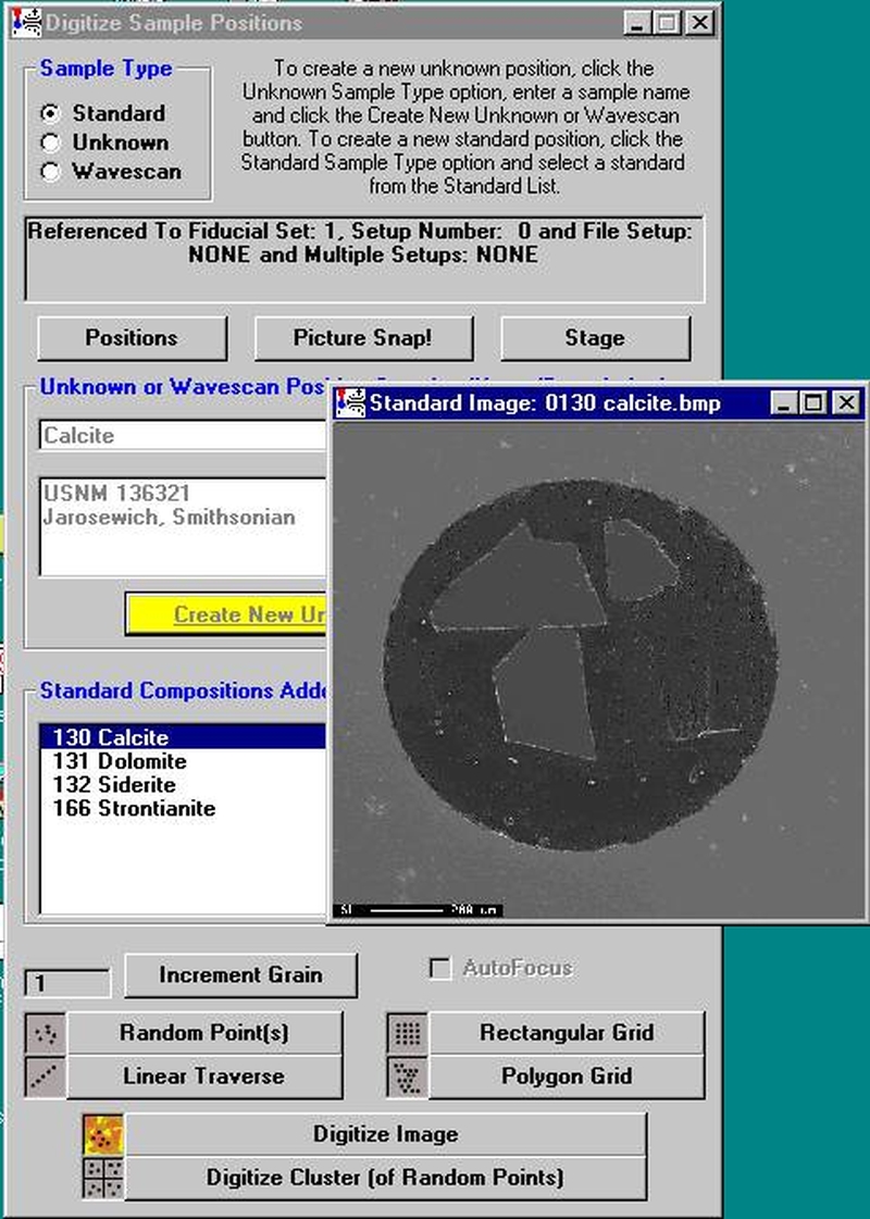
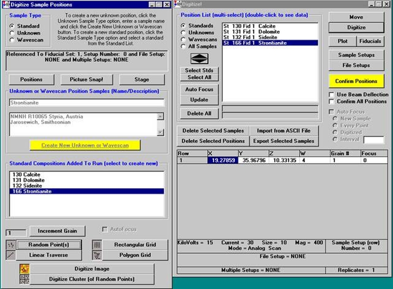
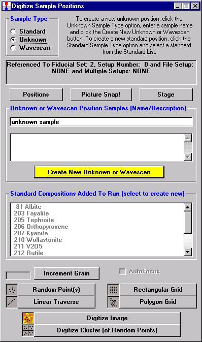
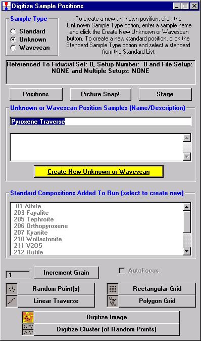
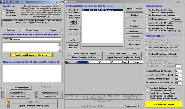
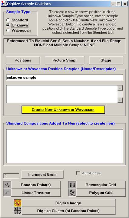
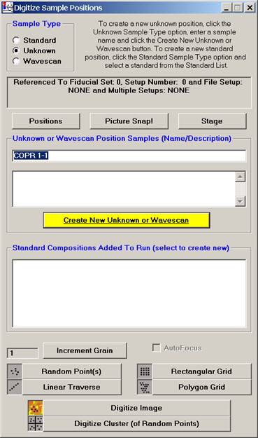
The Digitize Sample Positions window opens.
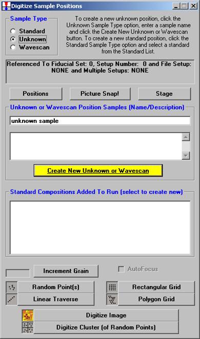
Select the Unknown check button from the Sample Type choices.
Enter a new sample name in the Unknown or Wavescan Position Samples text field, and click the Create New Unknown or Wavescan button.
A digitized polygon area grid will now be setup on the unknown grain.
Click the Polygon Grid button at the bottom of the Digitize Sample Positions window.
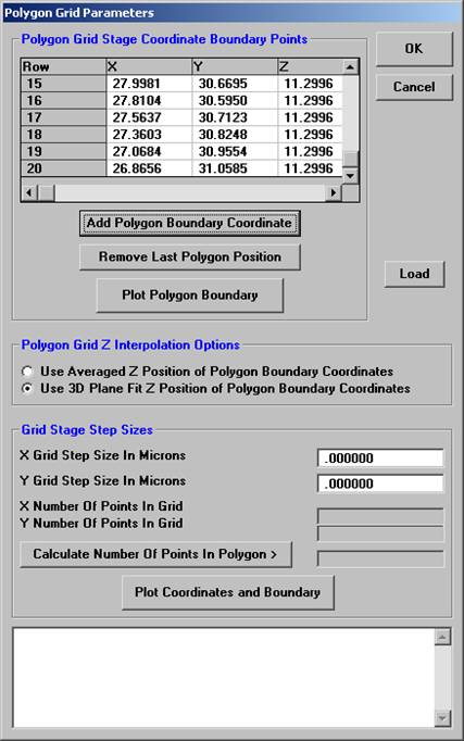
The Polygon Grid Parameters window opens.
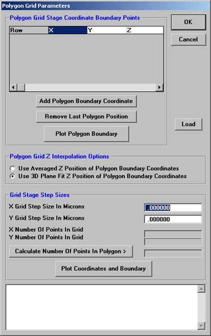
The user will outline the perimeter of the grain to be gridded. An easy way to accomplish this is to image the grain with backscattered electrons, at any magnification, and trace around the grain boundary. Start in one corner and on a recognizable feature, click the Add Polygon Boundary Coordinate button and then move linearly toward another feature or edge, clicking the Add Polygon Boundary Coordinate button to outline this portion of the grain. Continue to trace line segments around the grain, clicking the Add Polygon Boundary Coordinate button to enclose another portion of the grain. Eventually, returning to the starting point, completing the enclosure.
In this example, twenty line segments were used to enclose the grain of interest. Each end point is listed in the Polygon Grid Stage Coordinate Boundary Points text box. If a mistake is made or you simply wish to remove the previous boundary point, click the Remove Last Polygon Position button.
Click the Plot Polygon Boundary button to inspect the perimeter just drawn.
To start over and re-draw the perimeter outline again, click the Close button on the Polygon Plot window, click the Cancel button of the Polygon Grid Parameters window, and the click the Polygon Grid button of the Digitize Sample Positions window.
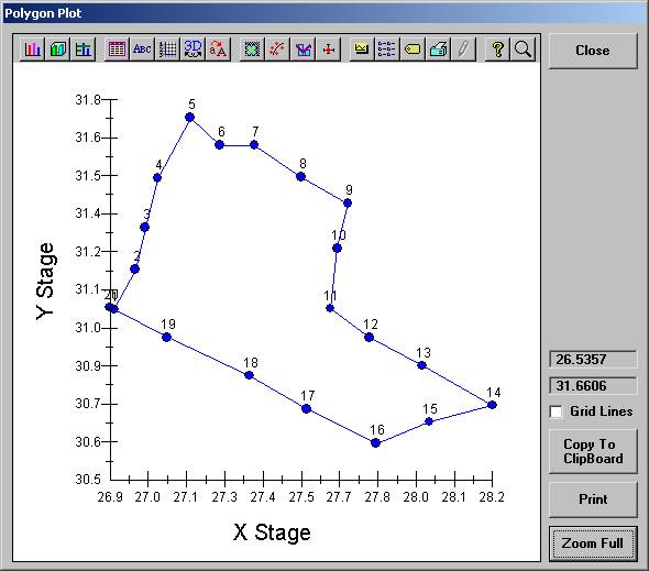
When satisfied with the outline of the grid, click the Close button of the Polygon Plot window.
Enter Grid Stage Step Sizes (in microns) for both X and Y.
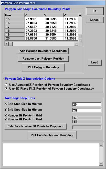
Click the Calculate Number of Points in Polygon> button to determine how many data points will be digitized. Readjust the X and Y Grid Step Sizes if necessary. Select a method of Z determination from the two option buttons under Polygon Grid Z Interpolation Options.
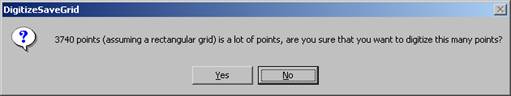
The DigitizeSaveGrid window appears with the number of points in an ideal rectangular grid.

Click the Yes button to calculate the total number of points.
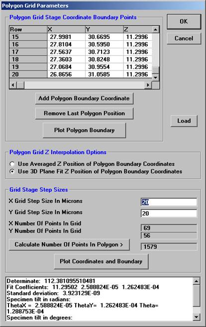
When the appropriate gridding parameters have been set, click the OK button, closing the Polygon Grid Parameters window.
The DigitizeSaveGrid window re-appears, click the Yes
button.
The program automatically digitizes each of the number of points in the polygon and returns to the Automate! window.

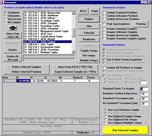
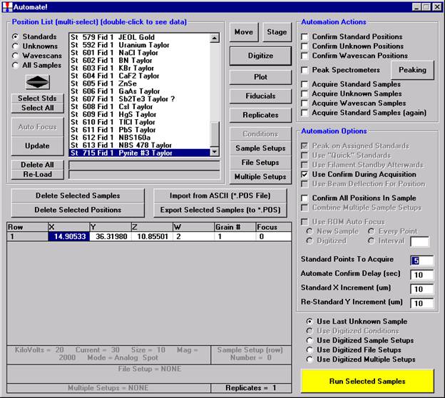
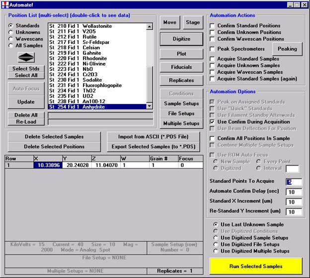
Click the Plot button in the Automate! dialog box to open the Position Plot window and view the locations of all of the digitized points in this sample. In this example, the 20 micron spacing creates too many points to be individually visible on this view.
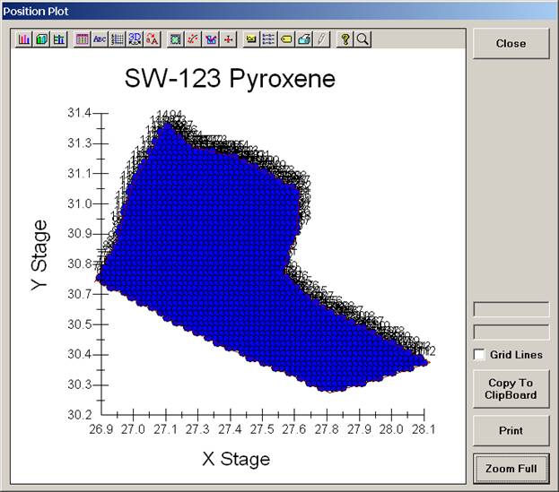
The user may click and drag the mouse to zoom on the plot to expand the scale.
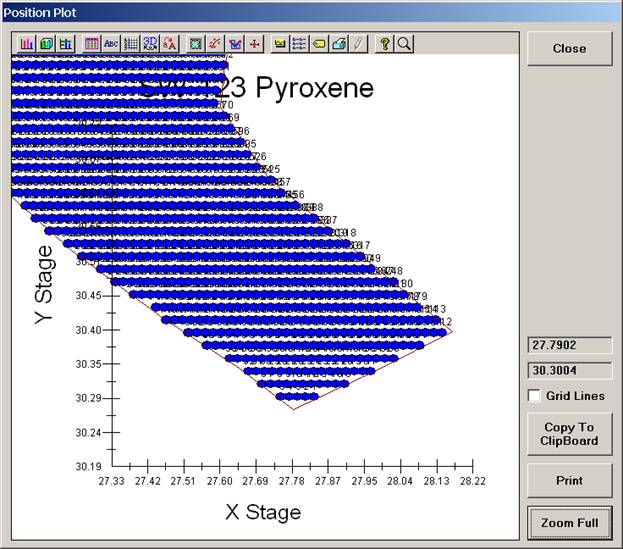
Click the Close button of the Position Plot window to return to the Automate! dialog box.
The user should proceed with calibration and standardization of the elements in the probe run and checking the accuracy of the standardization.
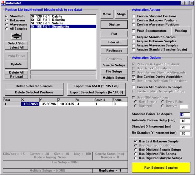
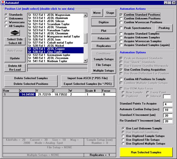
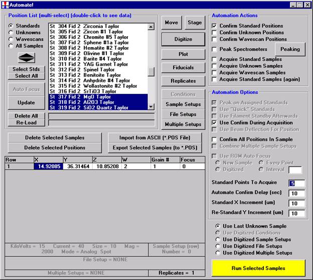
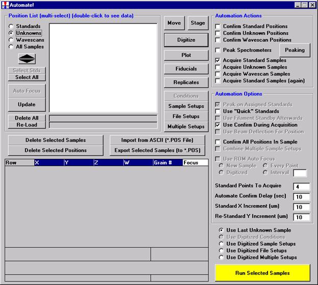
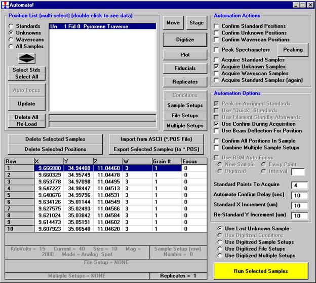
Then, to run the just digitized polygon grid sample from the Automate! window, highlight it in the Position List. Under the Automation Actions, click the Acquire Unknown Samples check box. Finally, click the Run Selected Samples button.
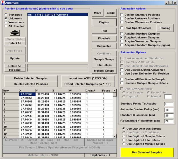
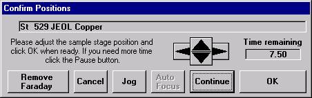
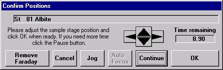
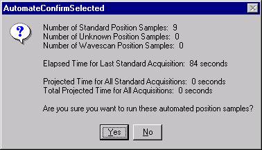
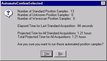
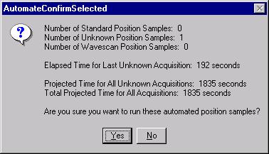
The AutomateConfirmSelected window opens and the user clicks the Yes button to activate the acquisition.
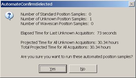
Note, acquisition time is now calculated.
Upon completion of the data acquisition, open the Plot! window.
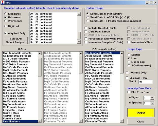
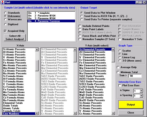
Select (highlight) all of the unknown digitized points (Un6-35 in this example). Click the Minimum Total check box to skip low points (analyses in holes, etc). Select the 3-D check button under Graph Type.
Click the Send Data to ASCII File check button. This activates the other check boxes listed here. Click the SURFER.BAS File check box and select an X-Axis, Y-Axis and Z-Axis (multi-select) parameters to plot.
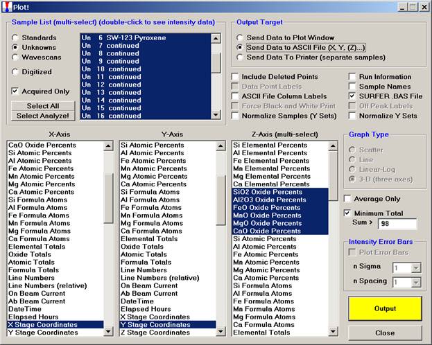
Click the Output button.
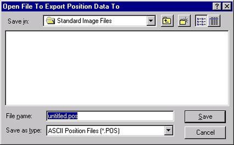
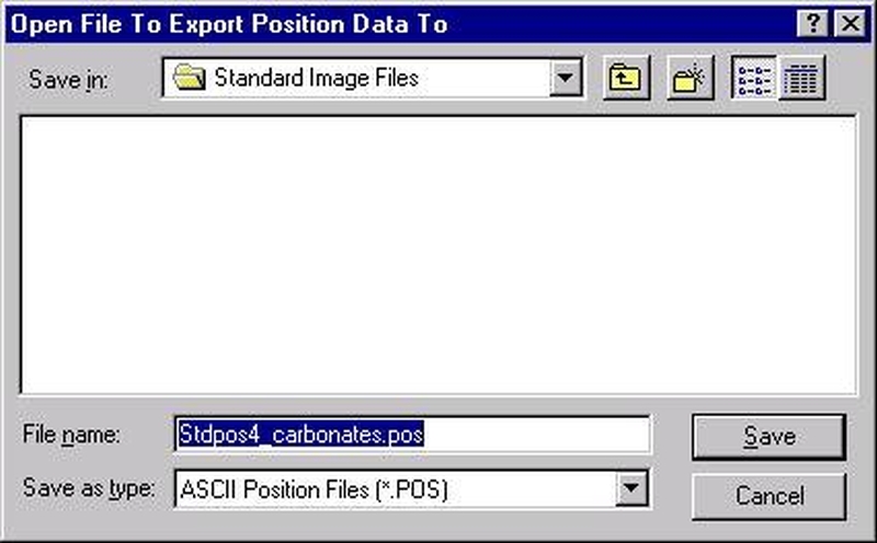
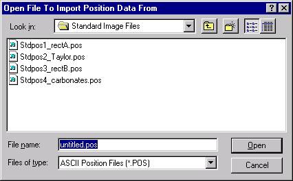
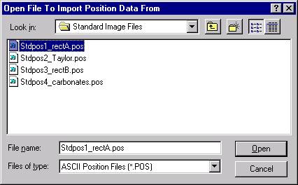
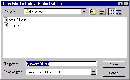
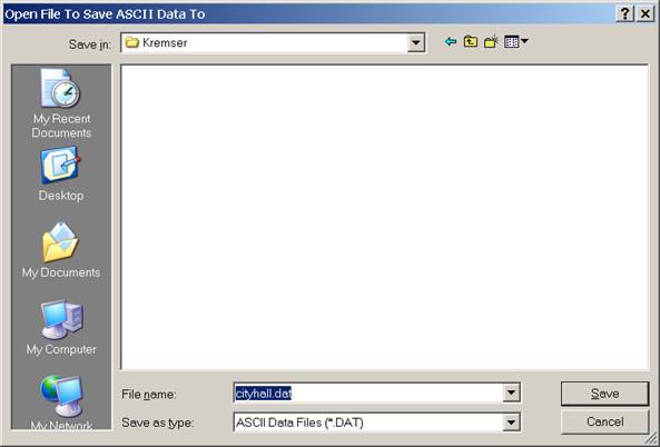
The Open File To Save ASCII Data To window opens. Adjust the Save in: location if required. Enter a File name: in the text field provided.
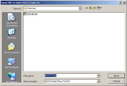
Click the Save button.
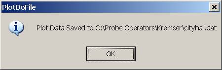
The PlotDoFile window opens, click the OK button.
Another PlotDoFile window appears.
Click the OK button to create these files.
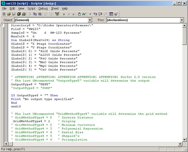
The SW123.BAS script file created above contains the OLE code for generating contour and surface plots of the digitized probe data.
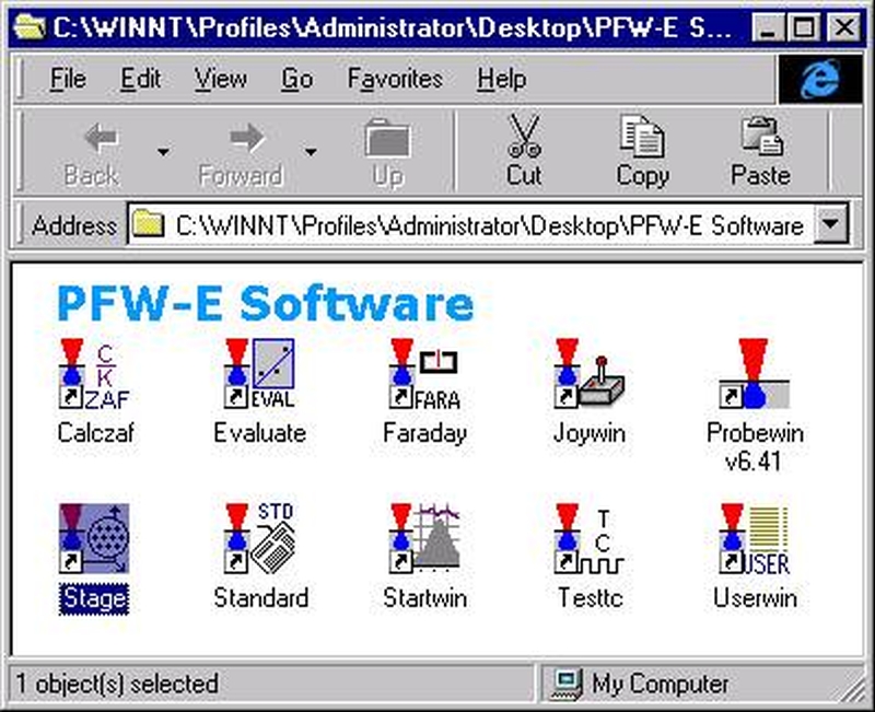
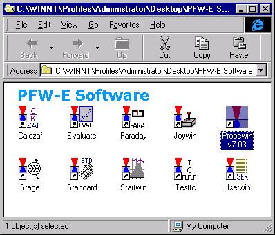
To run the SW123.BAS script file, double click on the GS Scripter32 icon in the EPMA Software folder on the desktop. Select the File | Open menu.
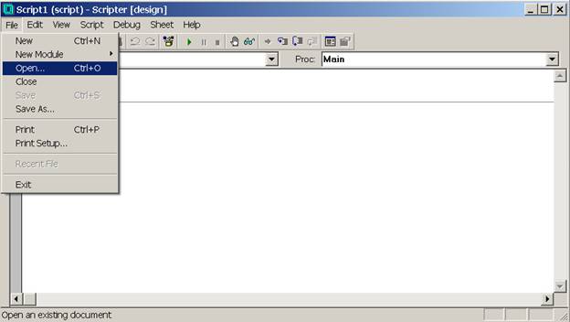
The Open Document window appears. Edit the Look in: directory to identify the location of the SW123.BAS file.
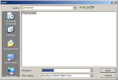
Click the Open button.
GS Scripter now details the open SW123.BAS file, of which a portion is illustrated below.
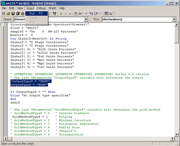
The default output mode of the script file is "TEST", which will only output the plots to the screen. To produce output to the default printer, comment out the line OutputType$ = "TEST" by placing a single quote in front of the line and uncomment the line OutputType$ = "SURF" by removing the single quote in front of it (highlighted in next screen capture).
Click Run | Start menu to begin the automated
plotting.
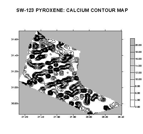
Basic contour and surface maps will be output to the printer. Raw data concentration (*.GRD) files will also be created; these may be opened in SURFER for further modification and output.
An example of a basic contour map for calcium is shown below. The perimeter of the pyroxene grain is visible. Regions of higher calcium concentrations appear dark in this view.
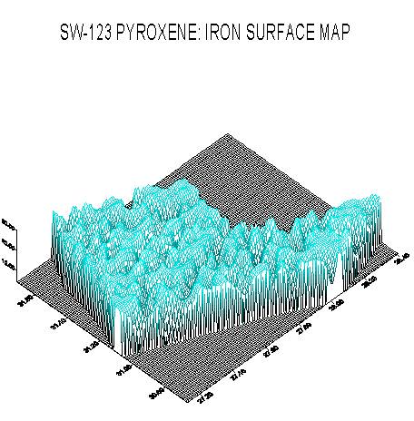
The next screen capture illustrates a 3-D surface map for iron in the pyroxene. Here, the image of iron concentration (vertical scale) has been rotated and tilted slightly.
Unknown or standard samples loaded into the electron microprobe can present some difficulty to the user in terms of rapid and precise positioning or the location of small phases or specific areas of interest to analyze upon a large sample. On the JEOL 733 microprobe the user has several options for searching for analysis or standard locations. An optical image (reflected or transmitted light) or a video feed of the same image is available but at only one relatively high magnification, about 400 times. Additionally, one can search for the area of interest utilizing the secondary or backscattered detectors on the microprobe at variable magnifications (ranging as low as 40 times), but this can be time consuming. Still the entire sample may not be in one field of view upon observation in the chamber.
Another device employed to aid in feature location and rapid positioning is a gridding device that holds a sample mounted in a standard holder under a moveable grid system. The rough coordinates of a region on the sample may be read off and used to effectively narrow the search for the analysis position.
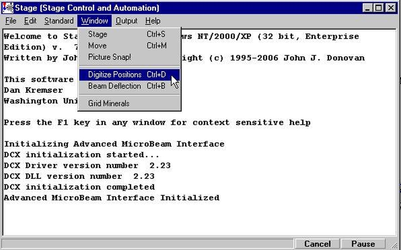
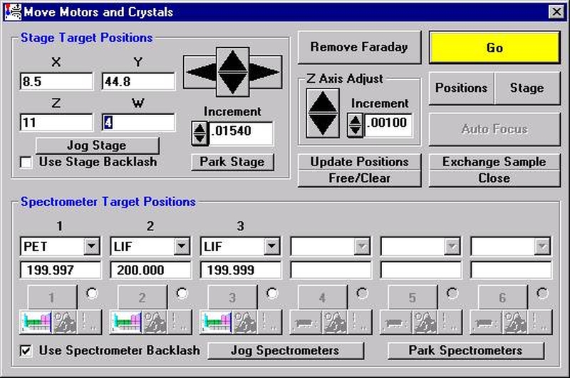
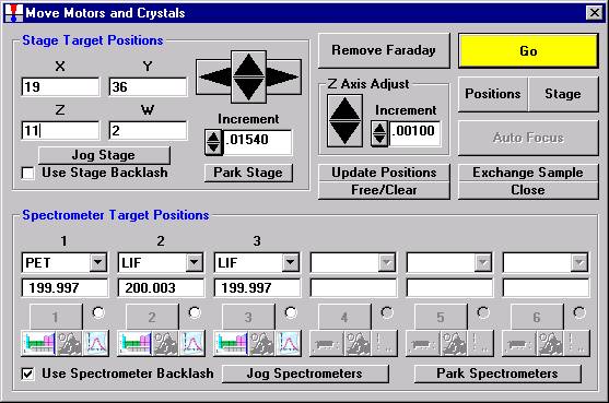
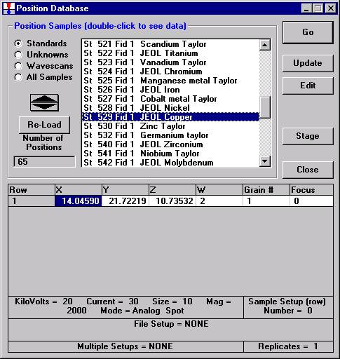
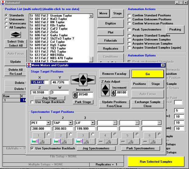
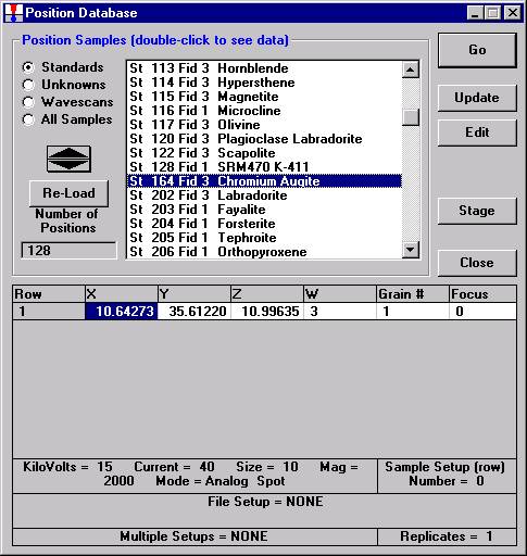
Now, navigation around and exact positioning is easily accomplished using the stage bit map and Picture Snap! features in PROBE FOR WINDOWS. The Stage Bit Map feature will be discussed first. The Stage button is located in the Move Motors and Crystals window.
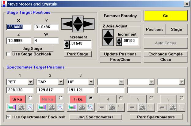
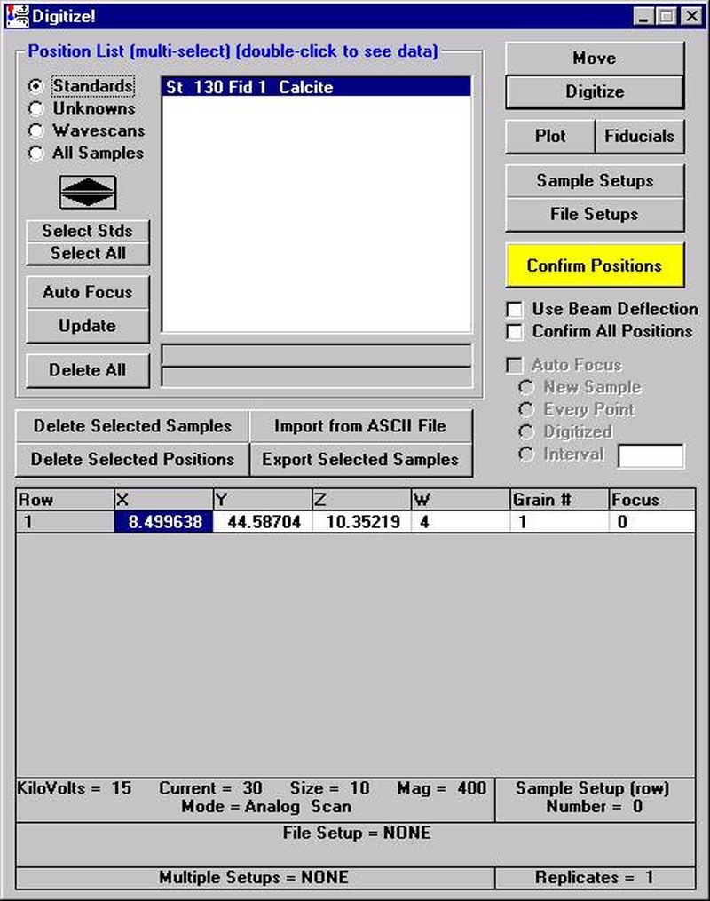
Clicking the Stage button opens the Stage Map window. Two different maps are displayed below.
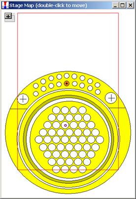
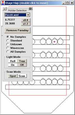
To select another Holder Selection image, simply select the file from the drop-down list box. Image files (windows metafiles (*.WMF)) and coordinate limits are specified in the Standards section of the PROBEWIN.INI file. The entire map maybe reduced or enlarged retaining scale using the x0.8 or x1.2 buttons or to re-size the Stage Bit Map window simply drag any corner of the window to the desired size and shape. The minus and plus button (upper left) minimizes the stage bitmap selection and cursor position display.
The current position is indicated as a small red-purple circle on the map. To move from one location to another, simply double-click on the spot you wish the stage to travel to. The current position (X and Y stage coordinates) is displayed above the Remove Faraday/ Insert Faraday button. Digitized positions of various samples can also be viewed by selecting the appropriate radio button.
To create stage drawing maps of your standard holders, for instance, use a vector based drawing program (Micrografx Designer or the shareware program Metafile Companion1) and the exact dimensions of your holders to build dimensionally correct drawings. These can be exported as windows metafiles and directly loaded into the graphical stage move feature in Probe for EPMA.
1Mention of specific third party software products does not imply their endorsement.
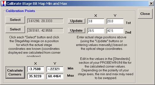
Each stage map must be calibrated in coordinate space for accurate movement to features on the map. Typically two diagonally located points near the edge of the map are chosen for calibration. Initiate the calibration routine by clicking the @ button (upper right) in the Stage Map window. The MoveStageMapCalibrate window appears.
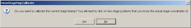
Click the Yes button to open the Calibrate Stage Bit Map Min and Max window for calibration.
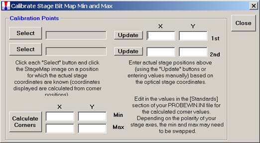
Click the top Select button, opening the Stage Select window.
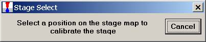
Click on the unique position on the stage map to identify the stage coordinates.
These values appear next to the Select button chosen.

Click the lower Select button and repeat the process. Click on the second position on the image. The Calibrate Stage Bit Map Min and Max window will appear as below.
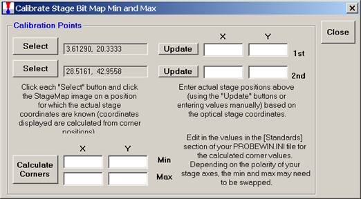
Next, enter the stage coordinate information (manually or by using the appropriate Update button) from the optical scanner or microscope coordinate system.
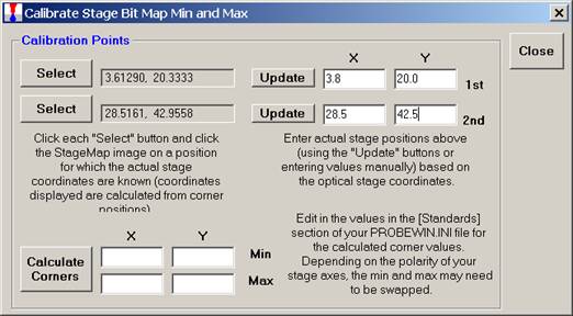
Click the Calculate Corners button to obtain the correct corner values to calibrate your Stage Map. These values min and max values are entered into the Standards section of the PROBEWIN.INI file.
The new Picture Snap! feature allows the user to incorporate images of your unknown thin section or polished mounts into PROBE FOR WINDOWS to aid in navigation and the digitizing of analysis locations. Images (BMP, JPEG, GRD) taken with a flatbed scanner or other camera system can be entered into Picture Snap!, then calibrated and used for analysis.
Picture Snap! dialog can be accessed from the Digitize Sample Positions window.
Picture Snap! can also be accessed from the STAGE program by accessing the Window | Picture Snap! menu.
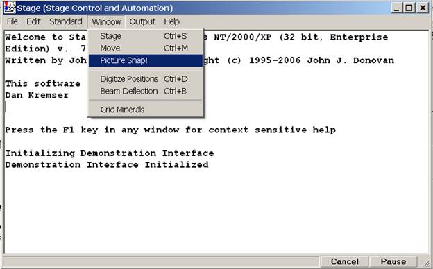
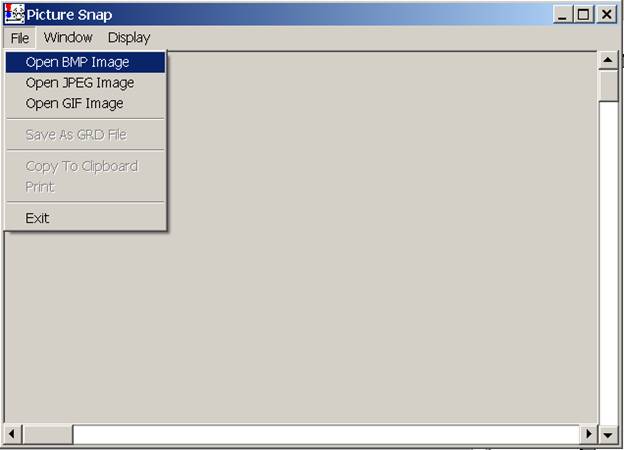
The main Picture Snap! window appears.
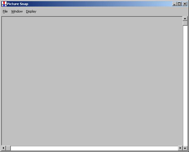
Select the File menu and open the appropriate image file.
The Open File To Input Bitmap Image From window opens.
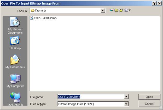
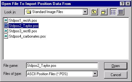
Select the appropriate directory and file to open and click the Open button.
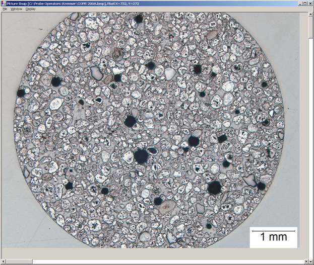
The image is displayed in the Picture Snap! window.
Select the Window | Calibrate menu.
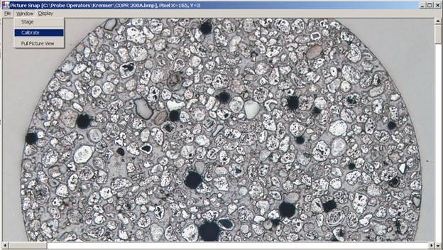
The Picture Snap Calibration window appears.
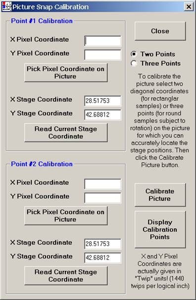
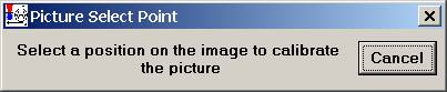
Image calibration is accomplished using a two point method for rectangular mounts or a three point calibration when importing round images subject to rotation. Click the Point #1 Calibration Pick Pixel Coordinate on Picture button The Picture Select Point window appears, select the first unique point on the image.
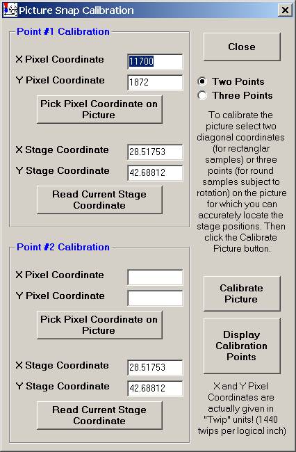
The X,Y Pixel Coordinates are entered.
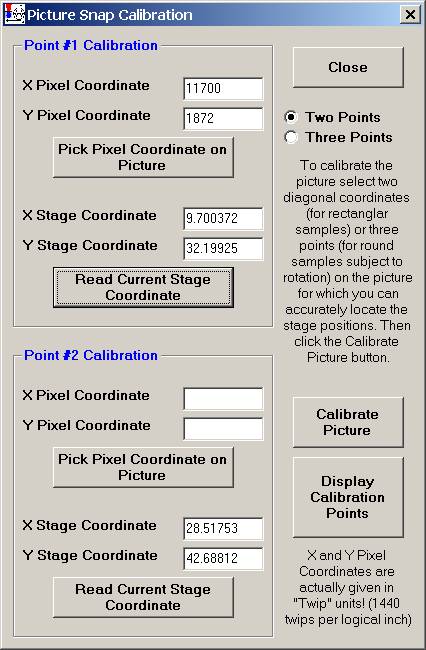
The values shown in the X, Y Stage Coordinates text boxes are the current stage location. Drive the stage to the same unique location and click the Read Current Stage Coordinate button.
The stage location for the first calibration point is entered.
Repeat these steps for the second calibration point, resulting in the following window.
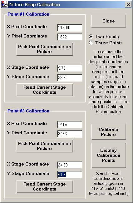
Finally, click the Calibrate Picture button opening the PictureSnapSaveCalibration window.
Click the OK button to save the picture calibration.
The operator can digitize analysis locations for later unattended work. Click the Digitize button.
This opens the familiar Digitize Sample Positions window.
Create a new unknown. Double click on the spot for the first analysis point on the just calibrated image to drive the stage to those coordinates. Click the Random Point(s) button to digitize that sample location. Additional points maybe saved. All analysis locations can be viewed from the Display | Unknown Position Samples menu. All analysis locations can be acquired via the Automate! Window.
Advanced Topics Section 2
Modal analysis is a statement of the composition of a sample expressed in terms of the relative amounts of phases or minerals present. These volumetric proportions can be estimated from quantitative measurements made on the specimen by point counting analysis. This quantitative modal analysis on unknown compositions is based on a defined set of modal phases, selected from a standard database. Any database of standard compositions may be used to define the phases.
There are three basic steps involved in the modal analysis routine. This procedure involves initially the acquisition of a large set of compositional data acquired using either multiple traverses or large area gridding. It is assumed that this data set is statistically representative of the sample. In the example illustrated below, a large representative area of a fine-grained sandstone thin section was gridded and some 324 quantitative analysis points were collected.
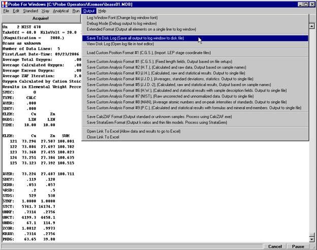
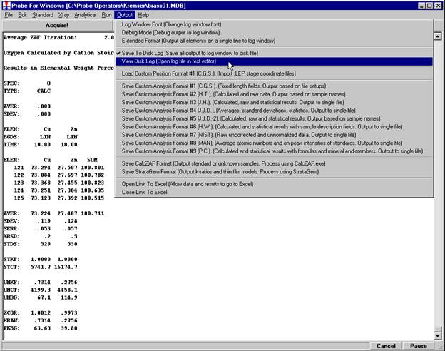
The second step involves the creation of an input file to load into STANDARD FOR WINDOWS for the actual modal analysis calculation. The simplest method of generating this input file is to use the Plot! window in Probe for EPMA to output a *.DAT file of the elemental or oxide weight percent compositions to disk.
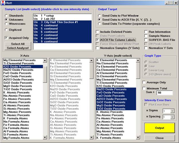
After data collection has been completed, open the Plot! window.
Highlight the compositional dataset in the Sample List.
Select the first oxide for the X-Axis and the remainder in the Y-Axis (multi-select) range.
Activate the Send Data to ASCII File (X, Y, (Z)…) check button and the ASCII File Column Labels check box. The labels are required so that the modal analysis routine can identify the elements in the input file.
The input file can come from any source as long as the element or oxide symbols are in the first line, enclosed within double quotes, and the data is in weight percent. The weight percent data can be in any format. Do not include a totals column.
Click the Output button.
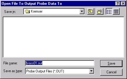
The Open File To Save ASCII Data To window appears. Locate the appropriate directory under Save in: and type in a File name: in the text field provided.
Click the Save button.
The PlotDoFile window appears, indicating that the data was saved.
Click the OK button.
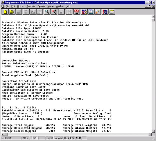
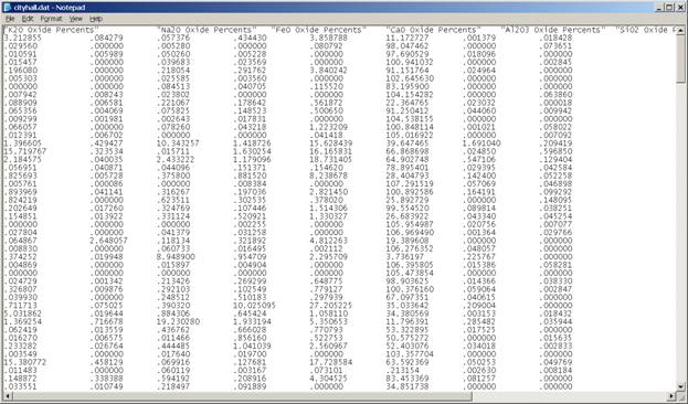
The data saved to the *.DAT file may be viewed using an editor such as Notepad. Here a portion of the CITYHALL.DAT file is displayed.
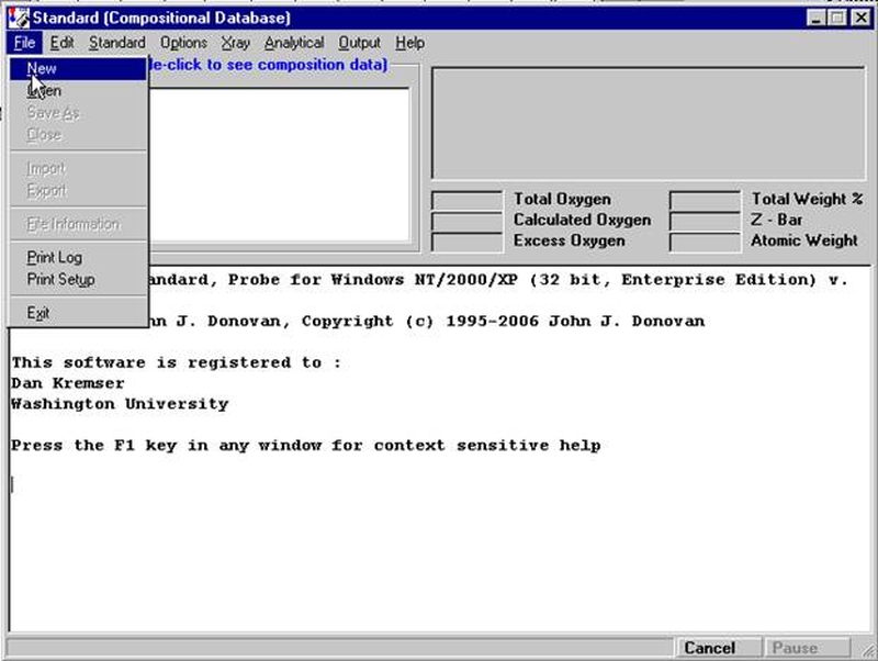
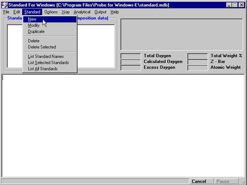
The third and final step involves the setup and running of the modal analysis calculation. The modal analysis routine is located in STANDARD FOR WINDOWS. Open the program Standard from the EPMA Software folder on the desktop.
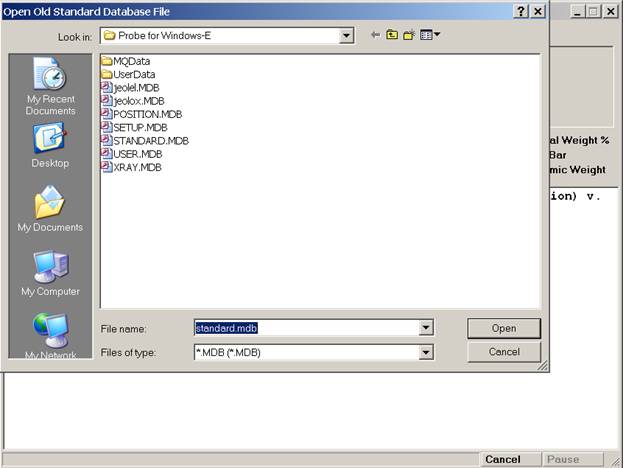
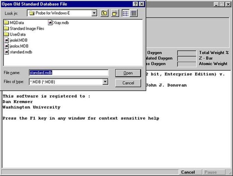
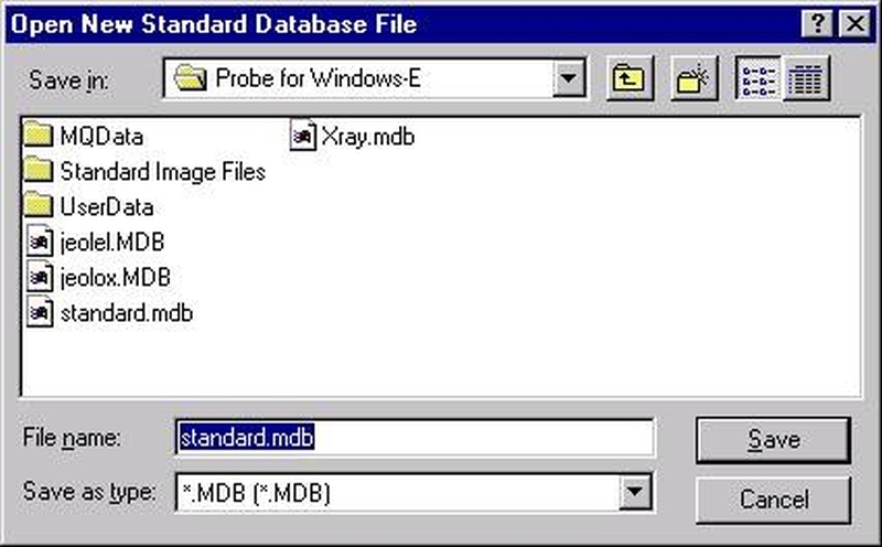
Select (highlight) a standard database that will be used to define the modal phases. Click the Open button to load this database.
Select Options | Modal Analysis from the menu.
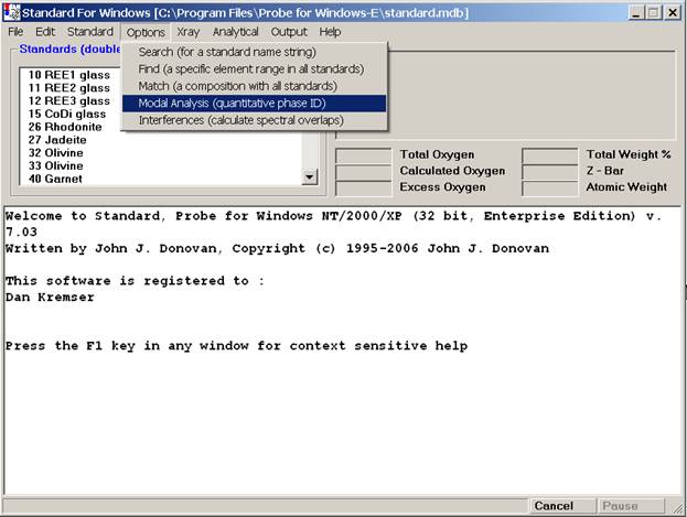
The Modal Analysis window opens.
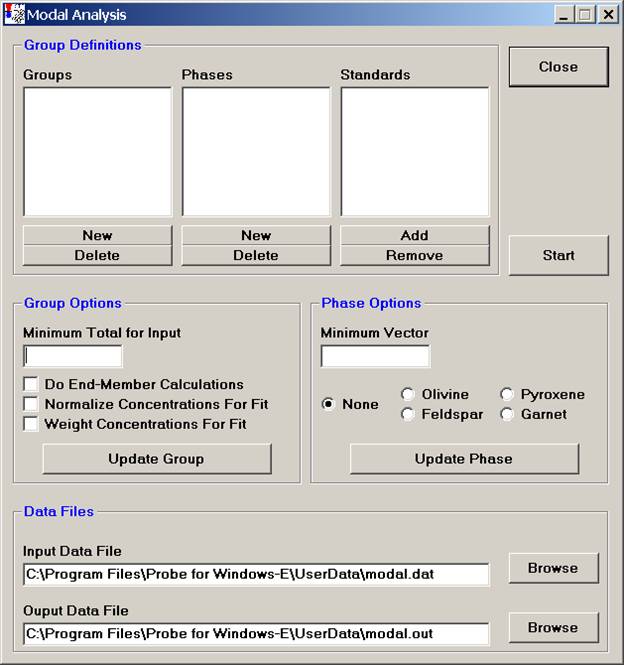
Start by defining an overall Group, click the New button under Groups.
The ModalGroupNew window opens. Enter a descriptive name for the group of phases.
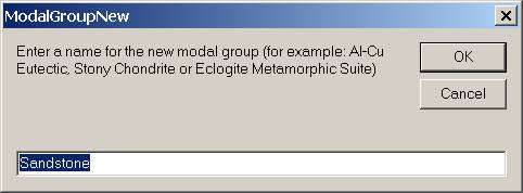
Click the OK button. Default Group and Phase Options are loaded; these will be discussed and modified shortly.
Click the New button under Phases.
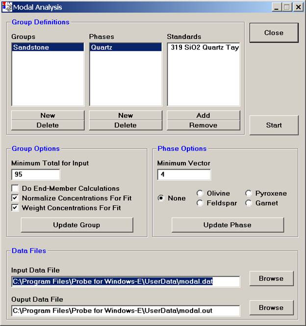
The ModalPhaseNew window opens. Enter the first modal phase. In this example, the sandstone is composed of mostly quartz with two minor feldspars; an alkali (sodium-potassium) phase and a plagioclase phase along with iron oxides and other trace accessory minerals. The first modal phase is entered into the text field.
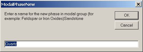
Click the OK button.
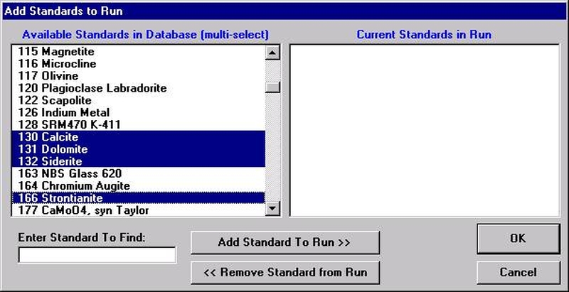
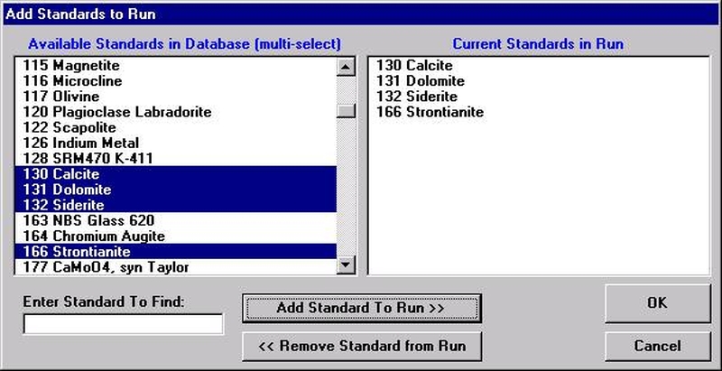
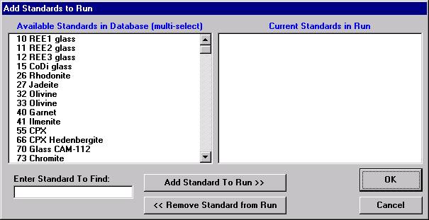
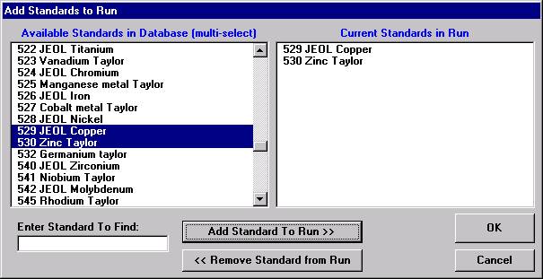
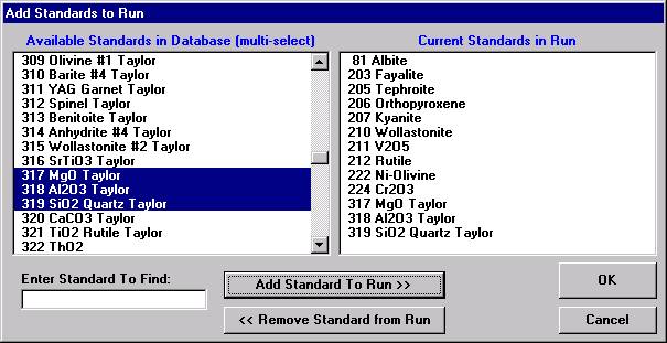
Select the Add button under Standards, opening the Add Standards to Run window.
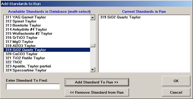
Choose standards to define this modal phase. These are the phase compositions that the program will use to match against the unknown point analyses. Try to avoid over-determining the phase. For example, when defining a sodium-potassium feldspar, select the two end-members (albite and microcline).
The Modal Analysis window would now appear as below.
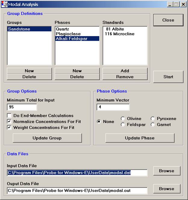
Continue and enter all phases, defining the phase compositions (standards) to match. The Alkali Feldspar entry is illustrated below.
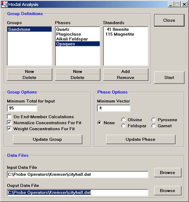
Once all of the phases have been identified and standards defined for matching, adjust the Group and Phase Options.

The Minimum Total for Input is the rejection sum for the unknown compositions, sums below this value will not be used in the modal analysis. Typically 90-95% are good cutoffs.
Select the Do End-Member Calculations option and check the appropriate mineral name under Phase Options to perform end-member calculations as listed.
The Normalize Concentrations For Fit option is used to specify whether the standard and unknown concentrations (above the just defined minimum input total) should be normalized to 100% before the vector fit is calculated.
The Weight Concentrations For Fit option is used to specify if the element concentrations for the standards should be weighted, based on the composition of the element in that phase. Select this option if the major elements in a phase should have greater influence in determining the vector fit. Leave unselected, if all concentrations, regardless of their abundance should have equal weight in the vector fit.
The Minimum Vector number (default is 4.0) is basically the tolerance for the match to a defined phase. If a closer match is desired for one or more phases in the group, decrease the vector value for that phase. See the User’s Guide and Reference documentation for specific details on the calculation of this vector.
Finally, under Data Files, select the appropriate Input and Output Data File locations.
Click the Start button to initiate the modal analysis calculation on each data point.
After the calculation finishes the ModalStartModal window appears, stating that the output data has been saved to the specified *.OUT file.
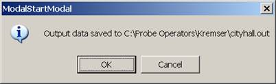
Click this OK button.
The modal analysis data may now be viewed in the log window in STANDARD FOR WINDOWS or simply open the newly created *.OUT file. The output file contains the vector fit, matched phase, end-member calculation (if checked), totals column and composition of each line in the input file. Lines that do not meet the minimum total requirement are excluded from the output, if those lines are desired either cut and paste the entire output from the main STANDARD FOR WINDOWS log window or capture the entire output by EARLIER selecting the Output | Save To Disk Log menu.
The results of the modal analysis are also tabulated and summarized. The end summary lists the total number of analyses, the minimum total for a valid composition, number of valid points that sum above the minimum sum, the number of matched points and the percentage of points that were matched.
For each phase, the summary output then lists the phase name, the number of matches for that phase, the percent of matched points, valid points and total matched points for the matches in that phase. This is followed by the average end-member (if selected), weight percent sum and composition for that phase and the standard deviation for each element.
The last page of the just run output file is displayed below.
Line  Vector  Phase     Sum     K2O    Na2O     FeO     CaO   Al2O3   SiO2     MgO    TiO2

268     .05  Quartz  100.30     .03     .02     .10     .10     .08   99.93     .00     .04
269     .04  Quartz   99.50     .02     .01     .12     .00     .12   99.17     .00     .06
270     .00  Quartz   99.66     .00     .00     .02     .00     .00   99.60     .00     .04
271     .06  Quartz   99.97     .02     .01     .20     .00     .12   99.62     .00     .00
272  ------  ------     .21     .04     .00     .00     .02     .03     .12     .01     .00
273     .00  Quartz   99.10     .01     .00     .02     .01     .00   99.04     .00     .02
274     .02  Quartz  100.07     .00     .00     .01     .00     .19   99.87     .00     .00
275     .02  Alkali   99.50     .23   11.50     .32     .03   18.85   68.57     .00     .00
276  ------  ------   36.50    5.25     .13    1.22    1.35    6.90   21.61     .04     .00
277     .00  Quartz   99.68     .00     .00     .01     .00     .00   99.68     .00     .00
278     .04  Quartz   98.30     .07     .00     .00     .03     .15   97.96     .03     .06
279  ------  ------     .13     .00     .00     .05     .02     .01     .06     .00     .00
280     .02  Quartz   99.17     .00     .00     .13     .03     .00   99.00     .01     .00
281     .06  Alkali   98.43   15.22     .24     .07     .01   18.23   64.65     .01     .00
282     .00  Quartz   99.79     .01     .00     .03     .00     .00   99.75     .00     .00
283     .01  Plagioc  98.09     .13     .02     .03   18.91   35.54   43.35     .07     .03
284     .00  Quartz   99.75     .00     .00     .04     .00     .00   99.68     .02     .01
285     .00  Quartz   99.59     .01     .00     .04     .00     .00   99.53     .02     .00
286     .67  Quartz   92.61     .07     .01     .29     .54     .16   91.46     .02     .06
287     .00  Quartz   99.43     .00     .00     .00     .03     .03   99.32     .00     .05
288     .02  Opaques  92.35     .03     .04   88.00     .01     .12     .42     .38    3.36
289  ------  ------   31.13     .23     .01     .15    1.66    1.45   27.55     .08     .00
290     .02  Quartz   99.65     .00     .00     .13     .00     .00   99.52     .00     .00
291     .13  Plagioc  99.23     .87     .08     .03   18.34   36.21   43.59     .09     .01
292  ------  ------   13.55     .04     .27     .07     .30     .19   12.55     .11     .03
293     .03  Plagioc  99.23     .03     .30     .12   18.88   36.27   43.54     .02     .07
294  ------  ------    9.42     .45     .00     .47     .56     .07    7.72     .00     .15
295  ------  ------   35.75     .30     .01     .61     .72   11.33   22.68     .09     .00
296  ------  ------     .86     .00     .00     .01     .01     .00     .85     .00     .00
297     .00  Quartz   99.88     .01     .00     .04     .01     .03   99.78     .00     .01
298     .21  Quartz   93.18     .13     .02     .20     .07     .20   92.48     .01     .07
299     .10  Quartz   98.14     .05     .03     .14     .12     .12   97.63     .03     .02
300     .00  Quartz  100.08     .00     .00     .04     .00     .00  100.05     .00     .00
301     .01  Quartz   99.49     .01     .00     .04     .02     .00   99.34     .02     .06
302     .02  Quartz  100.11     .00     .00     .08     .04     .00   99.91     .02     .07
303     .00  Quartz  100.32     .00     .00     .02     .02     .00  100.28     .00     .01
304     .00  Quartz   99.95     .00     .00     .00     .00     .00   99.95     .00     .00
305     .00  Quartz   99.97     .00     .00     .00     .00     .00   99.92     .00     .05
306     .02  Quartz  100.39     .01     .00     .09     .01     .00  100.21     .00     .06
307  ------  ------    7.62     .79     .00     .12     .33    1.09    5.27     .01     .00
308  ------  ------   15.00     .14     .01     .22     .22     .72   13.64     .04     .01
309  ------  ------    2.08     .06     .01     .14     .23     .36    1.26     .02     .00
310     .01  Plagioc  98.90     .14     .15     .01   19.20    35.63   43.65    .06     .06
311     .00  Quartz  101.36     .02     .00     .00     .02     .00   101.32    .00     .01
312     .02  Plagioc  99.02     .27     .01     .00   19.01   35.78    43.84    .11     .00
313  ------  ------   19.98     .32     .02    1.38    1.25    4.13   12.56     .30     .01
314  ------  ------   44.17     .04     .00     .15     .26   17.47   26.15     .01     .08
315  ------  ------    6.51     .00     .01     .05     .00     .10    6.34     .00     .00
316     .01  Quartz  100.85     .01     .00     .07     .00     .00  100.76     .00     .00
317  ------  ------     .40     .00     .00     .02     .02     .02     .32     .01     .01
318     .01  Quartz  100.95     .03     .00     .05     .02     .00  100.81     .04     .01
319     .00  Quartz  101.53     .00     .00     .03     .01     .00  101.46     .00     .03
320     .56  Quartz   98.51     .06     .00     .01     .33     .71   97.31     .07     .01
321     .01  Quartz  101.04     .02     .00     .07     .00     .00  100.92     .03     .00
322     .01  Quartz  101.03     .02     .00     .05     .02     .01  100.88     .00     .06
323     .00  Quartz  100.46     .00     .00     .00     .00     .00  100.45     .00     .01
324  ------  ------     .13     .00     .01     .02     .00     .00     .08     .00     .02

Results of Modal Analysis
InputFile : C:\Probe Operators\Kremser\cityhall.dat
OutputFile : C:\Probe Obrerators\Kremser\cityhall.out
Date and Time: 12/9/2006 9:42:46 AM
Group Name   : Sandstone
Total Number of points in File :  324
Valid Number of points in File :  240
Match Number of points in File :  237
Minimum Total for Valid Points :    90.00
Percentage of Valid Points :     74.1
Percentage of Match Points :     73.1

Phase   #Match  %Total  %Valid  %Match  AvgVec
Quartz     190    58.6    79.2    80.2     .09
           Sum     K2O    Na2O     FeO     CaO   Al2O3    SiO2     MgO    TiO2
Average: 99.27     .03     .01     .06     .04     .10   98.99     .01     .03
StdDev:   2.00     .08     .03     .08     .08     .21    2.12     .03     .03
Minimum: 90.60     .00     .00     .00     .00     .00   89.53     .00     .00
Maximum:102.77     .89     .34     .50     .54    1.52  101.46     .32     .20

Phase  #Match  %Total  %Valid  %Match  AvgVec
Plagiocl   20     6.2     8.3     8.4     .05
           Sum     K2O    Na2O     FeO     CaO   Al2O3    SiO2     MgO    TiO2
Average: 99.15     .31     .05     .08   18.73   36.01   43.90     .05     .02
StdDev:    .78     .34     .07     .10     .47     .28     .40     .03     .02
Minimum: 97.58     .02     .00     .00   17.95   35.54   43.32     .00     .00
Maximum:100.25    1.31     .30     .39   19.42   36.48   44.88     .11     .07

Phase  #Match  %Total  %Valid  %Match  AvgVec
AlkaliF    21     6.5     8.8     8.9     .06
           Sum     K2O    Na2O     FeO     CaO   Al2O3    SiO2     MgO    TiO2
Average: 99.11   13.19    1.83     .07     .22   18.40   65.33     .02     .03
StdDev:    .61    5.39    4.01     .07     .19     .28    1.50     .03     .04
Minimum: 97.60     .11     .02     .00     .01   18.02   63.91     .00     .00
Maximum:100.05   15.86   11.65     .32     .71   18.85   69.24     .08     .13

Phase  #Match  %Total  %Valid  %Match  AvgVec
Opaques6     1.9     2.5     2.5     .16
          Sum     K2O    Na2O     FeO     CaO   Al2O3    SiO2     MgO    TiO2
Average:91.69     .09     .05   88.86     .18     .39     .94     .43     .75
StdDev:  1.10     .07     .04     .64     .22     .46     .43     .33    1.31
Minimum:90.33     .01     .02   88.00     .00     .12     .42     .22     .03
Maximum:93.13     .18     .11   89.56     .59    1.29    1.38    1.09    3.36
Click the Close button on the Modal Analysis window.
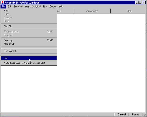
Finish by exiting STANDARD FOR WINDOWS.
This section describes how to calibrate the deadtime
constants for each spectrometer and where to enter them so that PROBE FOR
WINDOWS will utilize these factors.
Deadtime (τ) is defined as the time interval (after arrival of a pulse) when the counting system does not respond to additional incoming pulses (Reed, 1993). The equation normally used to correct for deadtime losses is given as:
 (1)
(1)
Where: n is the deadtime corrected count rate in counts per second
n' is the measured count rate in counts per second
τ is the deadtime constant in seconds
The time interval when the counting system is dead to additional pulses is defined as τn'. The live time then, is (1-τn'). The true count rate (n) is proportional to the beam current (i) by a constant factor, designated k. Thus, equation (1) may be rewritten as:
 (2)
(2)
A plot of n' / i (cps/nA) versus n' (cps) will yield a straight line with slope of (-kτ). The intercept on the n' / i axis will be the constant, k, and thus the deadtime factor (τ) may be determined.
A second deadtime correction option is also available in Probe for EPMA. This is a high precision expression for use with very high count rates (Willis, 1993). This expression differs from the normal equation only when very high count rates (>50K cps) are achieved. The precision deadtime expression is:
 (3)
(3)
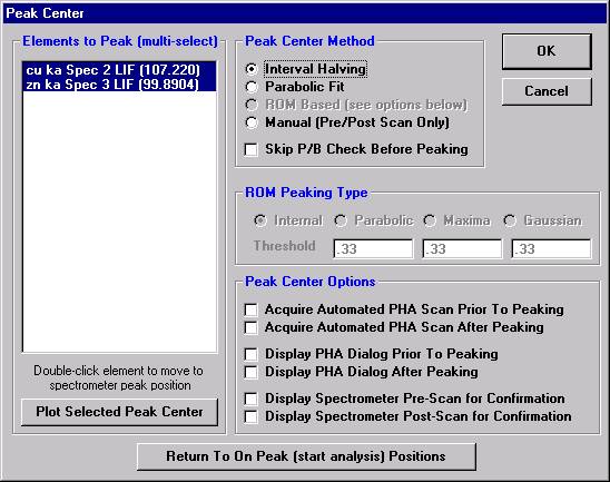
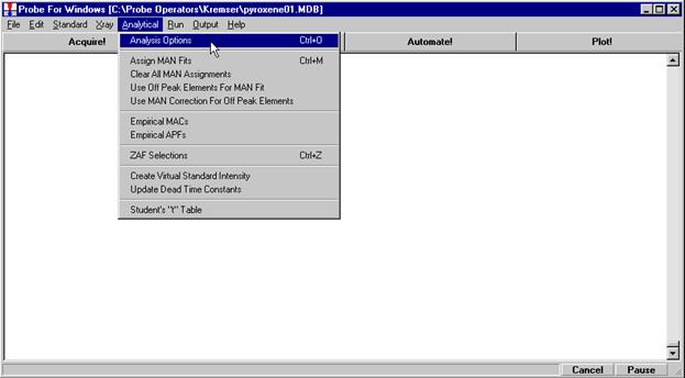
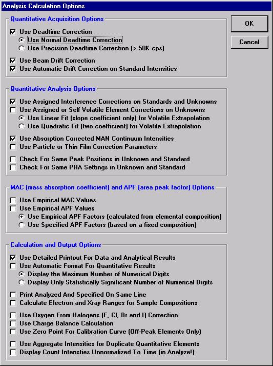
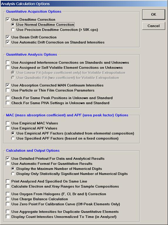
The deadtime correction option and type is selected from the Analysis Calculation Options window. Click Analytical | Analysis Options menu from the main Probe for EPMA log window. Click the OK button to confirm the selections.
STARTWIN can be used to obtain the x-ray intensities required for the deadtime calculation. The procedure involves collecting precise beam current and count rate data over a wide range of beam currents. This data set can then be loaded into the supplied Excel template to automatically calculate the deadtime factor for your spectrometers. Paul Carpenter has put together an excellent but slightly more elaborate Excel template, contact Probe Software, Inc. for further details on obtaining his spreadsheet and related documentation.
To calibrate the deadtime factors for your WDS system use high purity, homogeneous metal standards. Depending on the microprobe configuration one standard may be employed to collect data on all spectrometers. Here, a silicon metal standard will be used.
Open the Count Times window and disable both the Use Beam Drift Correction and the Normalize To Counts Per Second options to allow raw intensity data to be collected. Set an On Peak Count Time that will give a precise measurement of intensities.
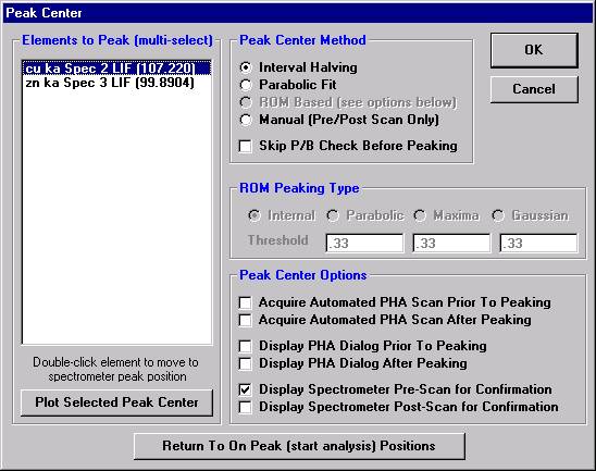
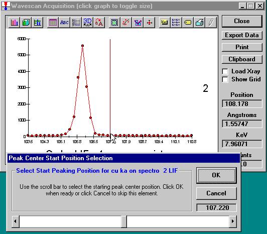
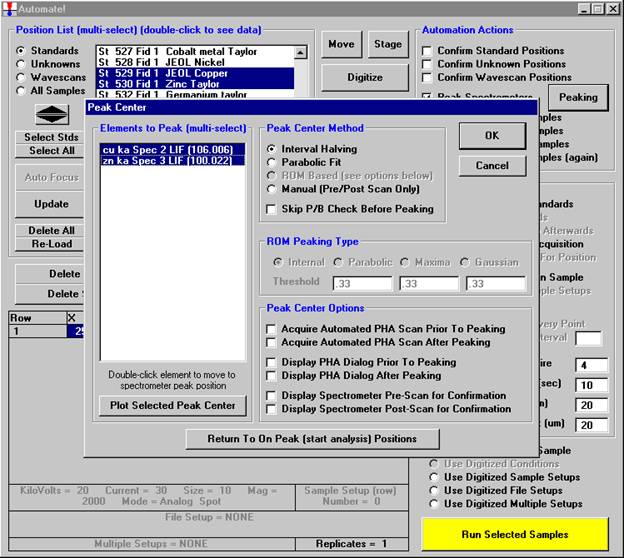
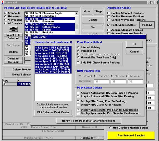
Peak each spectrometer to the x-ray line that will be used (Si Kα on TAP and Ti Kα on PET crystals for the JEOL). Upon completion of the peak center routine, move the spectrometers to the new peak positions.
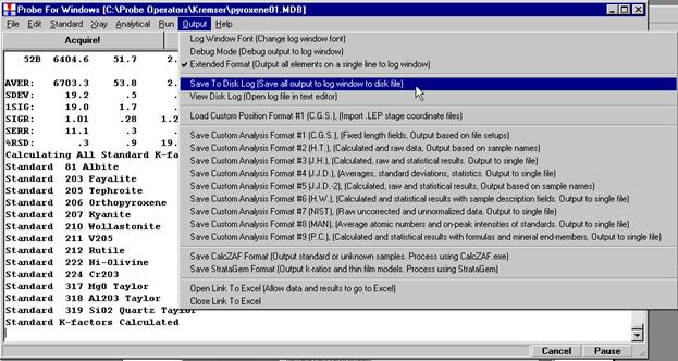
Prior to collecting data, run PHA scans on each spectrometer for Si Kα, check the pulse height distribution at low and very high beam currents (ideally duplicating the range of beam currents for the deadtime measurements). At very high count rates (large beam currents), significant pulse pileup and gain shifts do occur. Fully open your pulse height windows, optimize your gain settings to see all the signal over the range of beam currents employed.
Data collection and analysis is straightforward. Select Output | Open Link To Excel menu from the main STARTWIN log window. Collect three replicate intensity measurements and beam current data. Each time count rate data is acquired, it will automatically be sent to an Excel spreadsheet along with column labels. Measure the replicate count intensities at ten different beam currents; ranging from a few nanoamps to several hundred nanoamps.
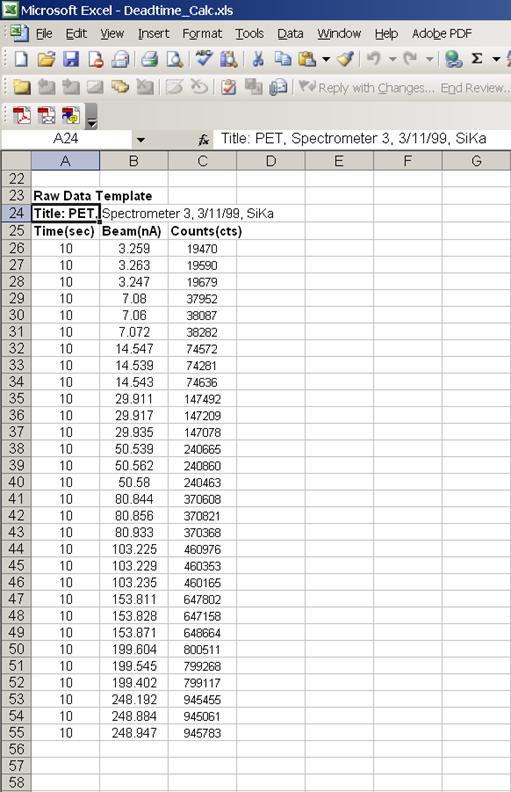
Create a count time column, prior to the beam current column in the Excel raw data spreadsheet and enter the relevant count times (in this example 10 seconds was used). The resulting spreadsheet may look similar to the one printed below except you may have data from more than three spectrometers.
Time	Beam	1	2	3
10	3.259	22083	79765	19470
10	3.263	22069	79995	19590
10	3.247	21755	80091	19679
10	7.08	42503	154130	37952
10	7.06	42642	154665	38087
10	7.072	42168	154182	38282
10	14.547	83163	293002	74572
10	14.539	83315	292602	74281
10	14.543	82998	293326	74636
10	29.911	162904	547744	147492
10	29.917	164053	549493	147209
10	29.935	163684	548386	147078
10	50.539	266841	838976	240665
10	50.562	266672	837625	240860
10	50.58	267751	837948	240463
10	80.844	409290	1169741	370608
10	80.856	410142	1169175	370821
10	80.933	409098	1168965	370368
10	103.225	507351	1352944	460976
10	103.229	507971	1354039	460353
10	103.235	508408	1352991	460165
10	153.811	709360	1640458	647802
10	153.828	711086	1640015	647158
10	153.871	710654	1641034	648664
10	199.604	873187	1790253	800511
10	199.545	871582	1788206	799268
10	199.402	873093	1788780	799117
10	248.192	1027320	1878180	945455
10	248.884	1027517	1878519	945061
10	248.947	1026681	1878716	945783
Open the DEADTIME_CALC.XLS file. Copy and paste count times, beam current information and counts for the first spectrometer into the raw data template starting in cell A26.
By placing data into this template, the program will automatically calculate the following items: the average of three replicate time counts, the average of three replicate beam current measurements, the %RSD on the average beam current, the average of three replicate raw intensity measurements and the %RSD on the average raw intensity measurement.
Next, the counts per second (x-axis) and the counts per second per nanoamp (y-axis) are determined. A least squares method is then used to calculate a straight line that best fits your data. The slope and Y-intercept are reported for a straight line fit to all 10 data pairs and also for the last 6. The latter being a more precise determination of deadtime.
Below is the calculation portion of the Excel template.
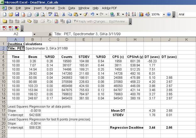
The following screen capture illustrates the raw data template.
Calculate the deadtime factor for each spectrometer in turn, by overwriting the last column of count data in the raw data template portion of the Excel spreadsheet. Simply highlight the data in the Excel linked spreadsheet (from STARTWIN), use the copy function and paste it into the appropriate column. Edit cells A2 and A24 to update the title of the spreadsheet, for documentation and printout purposes. Calculations on the new data set will be automatically updated and output.
The deadtime constants are placed into the SCALARS.DAT file (line 13). Enter a value for each spectrometer (units of microseconds, as output from the Excel spreadsheet).
Deadtime may not be a constant and probably varies with the line energy of the x-ray being measured. One way to get around this is to place a pulse stretching circuit before the counter timer board to ensure that a forced deadtime is used to mask the actual deadtime range of the spectrometer. A pulse width (from the pulse stretcher) greater than the worse case deadtime found for the spectrometer is produced. Using this value will lead to a more accurate deadtime correction at all energies.
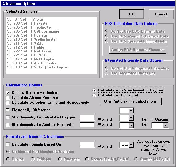
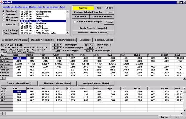
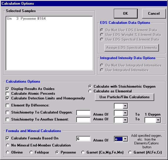
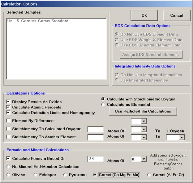
Prior to analyzing collected x-ray data, the user may wish to specify various output calculation options. These choices may be found by clicking the Calculation Options button in the Analyze! window.
The Calculation Options window opens.
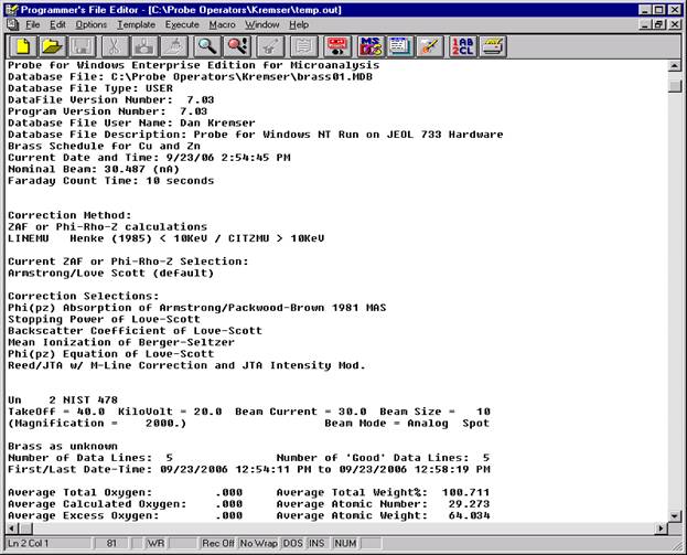
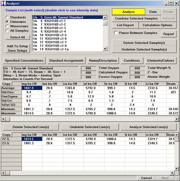
Each of the selected options in the above window will be briefly discussed in conjunction with the data output for the selected sample Un 5 Gore Mt. Garnet Standard.
Example Output Gore Mt. Garnet
Un    5 Gore Mt. Garnet Standard
TakeOff = 40.0  KiloVolt = 15.0  Beam Current = 30.0  Beam Size =    1
(Magnification =        .)                    Beam Mode = Analog  Spot

Std 40
Number of Data Lines:  2               Number of 'Good' Data Lines:  2
First/Last Date-Time: 11/21/1996 10:51:22 AM to 11/21/1996 10:55:35 AM

Average Total Oxygen:       42.298     Average Total Weight%:  100.752
Average Calculated Oxygen:  42.298     Average Atomic Number:   13.652
Average Excess Oxygen:        .000     Average Atomic Weight:   22.871
Average ZAF Iteration:        4.00     Average Quant Iterate:     2.00

Oxygen Calculated by Cation Stoichiometry and Included in the Matrix Correction

Results in Elemental Weight Percents

SPEC:        O
TYPE:     CALC

AVER:   42.298
SDEV:     .027

ELEM:       Mg      Mn      Ca      Al      Fe      Ti      Si
BGDS:      LIN     LIN     LIN     LIN     LIN     LIN     LIN
TIME:    40.00   40.00   40.00   40.00   40.00   40.00   20.00

ELEM:       Mg      Mn      Ca      Al      Fe      Ti      Si   SUM
    22   5.229    .418   5.345  11.932  17.024    .065  18.474 100.765
    23   5.189    .413   5.287  11.896  16.982    .067  18.588 100.740

AVER:    5.209    .415   5.316  11.914  17.003    .066  18.531 100.752
SDEV:     .028    .004    .041    .025    .029    .002    .081
SERR:     .020    .003    .029    .018    .021    .001    .057
%RSD:       .5      .9      .8      .2      .2     2.4      .4
STDS:       40      26      40      40      40      41      40

STKF:    .0330   .3086   .0499   .0841   .1468   .2898   .1370
STCT:   1818.5  1807.9  1356.0  5863.6   993.9  7261.9  2319.7

UNKF:    .0328   .0035   .0502   .0831   .1476   .0006   .1377
UNCT:   1807.9    20.8  1365.0  5792.0   999.3    14.5  2332.6
UNBG:     31.0     7.3    33.8    59.4    11.7    46.8     6.3

ZCOR:   1.5892  1.1716  1.0580  1.4339  1.1517  1.1330  1.3457
KRAW:    .9941   .0115  1.0066   .9878  1.0054   .0020  1.0055
PKBG:    59.27    3.87   41.44   98.54   86.43    1.31  375.63

Results in Oxide Weight Percents

SPEC:        O
TYPE:     CALC

AVER:     .000
SDEV:     .000

ELEM:      MgO     MnO     CaO   Al2O3     FeO    TiO2    SiO2   SUM
    22   8.671    .539   7.478  22.545  21.901    .108  39.522 100.765
    23   8.605    .533   7.398  22.478  21.848    .112  39.767 100.740

AVER:    8.638    .536   7.438  22.512  21.874    .110  39.645 100.752
SDEV:     .047    .005    .057    .048    .038    .003    .174
SERR:     .033    .003    .040    .034    .027    .002    .123
%RSD:       .5      .9      .8      .2      .2     2.4      .4

Results in Atomic Percents

SPEC:        O
TYPE:     CALC

AVER:   60.010
SDEV:     .026

ELEM:       Mg      Mn      Ca      Al      Fe      Ti      Si   SUM
    22   4.884    .173   3.027  10.040   6.921    .031  14.933 100.000
    23   4.846    .170   2.994  10.007   6.902    .032  15.021 100.000

AVER:    4.865    .172   3.011  10.023   6.911    .031  14.977 100.000
SDEV:     .027    .001    .024    .023    .013    .001    .063
SERR:     .019    .001    .017    .017    .009    .001    .044
%RSD:       .6      .9      .8      .2      .2     2.3      .4


Results Based on 24 Atoms of o

SPEC:        O
TYPE:     CALC

AVER:   24.000
SDEV:     .000

ELEM:       Mg      Mn      Ca      Al      Fe      Ti      Si   SUM
    22   1.954    .069   1.211   4.016   2.769    .012   5.974  40.005
    23   1.937    .068   1.197   4.001   2.759    .013   6.006  39.981

AVER:    1.946    .069   1.204   4.009   2.764    .012   5.990  39.993
SDEV:     .012    .001    .010    .011    .007    .000    .022
SERR:     .008    .000    .007    .008    .005    .000    .016
%RSD:       .6      .9      .8      .3      .2     2.3      .4

Garnet Mineral End-Member Calculations (Ca, Mg, Fe, Mn)

           Gro     Pyr     Alm      Sp
    22    20.2    32.6    46.1     1.2
    23    20.1    32.5    46.3     1.1

AVER:     20.1    32.5    46.2     1.1
SDEV:       .1      .0      .1      .0

Detection limit at 99 % Confidence in Elemental Weight Percent (Single Line):

ELEM:       Mg      Mn      Ca      Al      Fe      Ti      Si
    22    .012    .039    .017    .012    .043    .023    .023
    23    .012    .041    .017    .012    .044    .023    .020

AVER:     .012    .040    .017    .012    .044    .023    .021
SDEV:     .000    .001    .000    .000    .001    .000    .002
SERR:     .000    .001    .000    .000    .000    .000    .001

Percent Analytical Error (Single Line):

ELEM:       Mg      Mn      Ca      Al      Fe      Ti      Si
    22      .4     5.1      .4      .2      .5    14.6      .5
    23      .4     5.3      .4      .2      .5    14.4      .5

AVER:       .4     5.2      .4      .2      .5    14.5      .5
SDEV:       .0      .1      .0      .0      .0      .2      .0
SERR:       .0      .1      .0      .0      .0      .1      .0

Range of Homogeneity in +/- Elemental Weight Percent (Average of Sample):

ELEM:       Mg      Mn      Ca      Al      Fe      Ti      Si
  60ci    .025    .004    .035    .023    .025    .001    .077
  80ci    .055    .009    .078    .052    .056    .003    .172
  90ci    .113    .019    .159    .107    .114    .007    .353
  95ci    .228    .038    .321    .214    .230    .014    .710
  99ci   1.142    .189   1.607   1.074   1.151    .069   3.556

Test of Homogeneity at 1.0 % Precision (Average of Sample):

ELEM:       Mg      Mn      Ca      Al      Fe      Ti      Si
  60ci     yes     yes     yes     yes     yes      no     yes
  80ci      no      no      no     yes     yes      no     yes
  90ci      no      no      no     yes     yes      no      no
  95ci      no      no      no      no      no      no      no
  99ci      no      no      no      no      no      no      no


Level of Homogeneity in +/- Percent (Average of Sample):

ELEM:       Mg      Mn      Ca      Al      Fe      Ti      Si
  60ci      .5     1.0      .7      .2      .1     2.3      .4
  80ci     1.1     2.2     1.5      .4      .3     5.1      .9
  90ci     2.2     4.5     3.0      .9      .7    10.4     1.9
  95ci     4.4     9.1     6.0     1.8     1.4    21.0     3.8
  99ci    21.9    45.5    30.2     9.0     6.8   105.2    19.2

Detection Limit in Elemental Weight Percent (Average of Sample):

ELEM:       Mg      Mn      Ca      Al      Fe      Ti      Si
  60ci     ---    .008     ---     ---     ---    .008     ---
  80ci     ---    .017     ---     ---     ---    .018     ---
  90ci     ---    .035     ---     ---     ---    .037     ---
  95ci     ---    .070     ---     ---     ---    .075     ---
  99ci     ---    .349     ---     ---     ---    .374     ---

Projected Detection Limits (99% CI) in Elemental Weight Percent (Average of Sample):

ELEM:       Mg      Mn      Ca      Al      Fe      Ti      Si
TIME:      .63     .63     .63     .63     .63     .63     .31
PROJ:      ---   2.793     ---     ---     ---   2.989     ---
TIME:     1.25    1.25    1.25    1.25    1.25    1.25     .63
PROJ:      ---   1.975     ---     ---     ---   2.113     ---
TIME:     2.50    2.50    2.50    2.50    2.50    2.50    1.25
PROJ:      ---   1.396     ---     ---     ---   1.494     ---
TIME:     5.00    5.00    5.00    5.00    5.00    5.00    2.50
PROJ:      ---    .987     ---     ---     ---   1.057     ---
TIME:    10.00   10.00   10.00   10.00   10.00   10.00    5.00
PROJ:      ---    .698     ---     ---     ---    .747     ---
TIME:    20.00   20.00   20.00   20.00   20.00   20.00   10.00
PROJ:      ---    .494     ---     ---     ---    .528     ---
TIME:    40.00   40.00   40.00   40.00   40.00   40.00   20.00
PROJ:      ---    .349     ---     ---     ---    .374     ---
TIME:    80.00   80.00   80.00   80.00   80.00   80.00   40.00
PROJ:      ---    .247     ---     ---     ---    .264     ---
TIME:   160.00  160.00  160.00  160.00  160.00  160.00   80.00
PROJ:      ---    .175     ---     ---     ---    .187     ---
TIME:   320.00  320.00  320.00  320.00  320.00  320.00  160.00
PROJ:      ---    .123     ---     ---     ---    .132     ---
TIME:   640.00  640.00  640.00  640.00  640.00  640.00  320.00
PROJ:      ---    .087     ---     ---     ---    .093     ---
TIME:  1280.00 1280.00 1280.00 1280.00 1280.00 1280.00  640.00
PROJ:      ---    .062     ---     ---     ---    .066     ---
TIME:  2560.00 2560.00 2560.00 2560.00 2560.00 2560.00 1280.00
PROJ:      ---    .044     ---     ---     ---    .047     ---

Analytical Sensitivity in Elemental Weight Percent (Average of Sample):

ELEM:       Mg      Mn      Ca      Al      Fe      Ti      Si
  60ci    .035    .006    .049    .033    .035    .002    .109
  80ci    .078    .013    .110    .073    .079    .005    .243
  90ci    .160    .027    .225    .151    .161    .010    .499
  95ci    .322    .053    .454    .303    .325    .020   1.004
  99ci   1.615    .267   2.272   1.519   1.628    .098   5.029
Selecting Display Results As Oxides check box permits the user to display the results of an analysis in oxide weight percents based on the cation ratios defined for each element in the Element/Cations dialog window. Results are also, always reported in elemental weight percents.
The Calculate with Stoichiometric Oxygen button allows the user to calculate oxygen by stoichiometry if oxygen is not an analyzed element in the routine. If oxygen is either measured or calculated by stoichiometry and the Display Results As Oxides check box is selected, then the program will automatically calculate and report the actual excess or deficit oxygen in the analysis. This information can be very useful in determining if the selected cation ratios are correct (iron bearing oxides, for example).
All elements to be calculated by stoichiometry, difference or formula basis must be listed in the sample setup. Add these elements using the Elements/Cations button. Each must be added as a “not analyzed” element; click any empty row in the element list, type in the element symbol and leave the x-ray line blank. Analyses can also be output as atomic percents if the Calculate Atomic Percents check box is marked. This calculation is based on the fraction of the atomic weight of each element and is normalized to a 100% total.
The Formula and Mineral Calculation fields at the base of the Calculation Options window allow the user to compute formulas based on any number of oxygens for oxide runs or any analyzed or specified element in elemental runs. Further, olivine, feldspar, pyroxene, and two garnet end-member calculations are written into the software. These formula calculations are based only on atomic weight and do not consider charge balance and site occupancy. See the appendix sections in An introduction to The Rock-Forming Minerals by Deer, Howie, and Zussman (1992) for details on calculating formulas for hydrous phases.
The user may also select the Calculate Detection Limits and Homogeneity check box. The calculation of the sample detection limits is based on the standard counts, the unknown background counts, and includes the magnitude of the ZAF correction factor. The calculation is adapted from Scott et al., (1995). This detection limit calculation is useful in that it can be used even on inhomogenous samples and can be quoted as the detection limit in weight percent for a single analysis line with a confidence of 99% (assuming 3 standard deviations).
Where:
ZAF is the ZAF correction factor for the sample matrix
IS is the count rate on the analytical (pure element) standard
IB is the background count rate on the unknown sample
t is the counting time on the unknown sample
After this, a rigorous calculation of the analytical error also for single analysis lines, is performed based on the peak and background count rates (Scott et al., 1995). The results of the calculation are displayed after multiplication by a factor of 100 to give a percent analytical error of the net count rate. This analytical error result can be compared to the percent relative standard deviation (%RSD) displayed in the analytical calculation. The analytical error calculation is as follows:

Where:
NP is the total peak counts
NB is the total background counts
tP is the peak count time
tB is the background count time
A more comprehensive set of calculations for analytical statistics will also be performed. These statistics are based on equations adapted from Scanning Electron Microscopy and X-Ray Microanalysis, Second Edition by Goldstein, et al., (1992). All calculations are expressed for various confidence intervals from 60 to 99% confidence.
The calculations are based on the number of data points acquired in the sample and the measured standard deviation for each element. This is important because although x-ray counts theoretically have a standard deviation equal to square root of the mean, the actual standard deviation is usually larger due to variability of instrument drift, x-ray focusing errors, and x-ray production.
The statistical calculations include:
The range of homogeneity in plus or minus weight percent.
The level of homogeneity in plus or minus percent of the concentration.

The trace element detection limit in weight percent.
The analytical sensitivity in weight percent.

Where:
 is the concentration to be compared with
C is the actual concentration in weight percent of the sample
Cs is the actual concentration in weight percent of the standard
 is the Student tfor a 1-α confidence and n-1 degrees of freedom
n is the number of data points acquired
 is the standard deviation of the measured values
 is the average number of counts on the unknown
 is the continuum background counts on the unknown
 is the average number of counts on the standard
 is the continuum background counts on the standard
The homogeneity test compares the 99% confidence range of homogeneity value with 1% of the sample concentration for each element. If the range of homogeneity is less than 1% of the sample concentration then the sample may be considered to be homogenous within 1%. The detection limit calculation here is intended only for use with homogenous samples since the calculation includes the actual standard deviation of the measured counts. This detection limit can, however, be quoted for the sample average and of course will improve as the number of data points acquired increases. Note that the homogenous sample detection limit calculation are ignored for those elements which occur as minor or major concentrations (>1%).
Conversely, the analytical sensitivity calculation is ignored for elements whose concentrations are present at less than 1%.
Three other calculation options are available to the user; Element By Difference, Stoichiometry To Calculated Oxygen, and Stoichiometry To Another Element.
When the Element By Difference check box is selected, the user can include an element in the analysis to account for their affect on the other x-ray intensities. This element must be specified in the sample setup. Note this method causes the calculation to result in a 100% total.
The Stoichiometry To Calculated Oxygen option is often used in the analysis of carbonate or borate samples in an oxide run. This feature permits the user to analyze just the cations in the sample and have oxygen calculated by stoichiometry and another specified element (usually C in carbonates and B in borates) calculated relative to oxygen. In the carbonate scenario (CaCO3), carbon is always in the ratio of 1 to 3 to oxygen. If the user specifies carbon by stoichiometry relative to the stoichiometric element oxygen at 0.333 (1 divided by 3) the correct amount of both carbon and oxygen will be incorporated into the ZAF matrix correction and totals without analyzing for either element. This method should only be used with phases where the ratio to oxygen is both fixed and known.
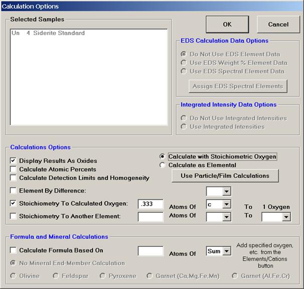
The following iron carbonate mineral (siderite) output illustrates oxygen calculated by cation stoichiometry with the element carbon is calculated at 0.333 atoms relative to 1.0 atom of oxygen.
Un    4 Siderite Standard
TakeOff = 40.0  KiloVolt = 15.0  Beam Current = 15.0  Beam Size =   10
(Magnification =        .)                    Beam Mode = Analog  Spot
Number of Data Lines:  3               Number of 'Good' Data Lines:  3
First/Last Date-Time: 07/26/1999 02:45:52 PM to 07/26/1999 02:51:12 PM

Average Total Oxygen:       41.449     Average Total Weight%:  100.042
Average Calculated Oxygen:  41.449     Average Atomic Number:   16.438
Average Excess Oxygen:        .000     Average Atomic Weight:   23.164
Average ZAF Iteration:        8.00     Average Quant Iterate:     2.00

Oxygen Calculated by Cation Stoichiometry and Included in the Matrix Correction
Element C is Calculated  .333 Atoms Relative To 1.0 Atom of Oxygen

Results in Elemental Weight Percents

SPEC:        C       O
TYPE:     STOI    CALC

AVER:   10.356  41.449
SDEV:     .017    .013

ELEM:       Ca      Mg      Mn      Fe
BGDS:      LIN     LIN     LIN     LIN
TIME:    20.00   30.00   40.00   40.00

ELEM:       Ca      Mg      Mn      Fe   SUM
    19    .000    .067   2.235  45.825  99.929
    20    .014    .072   2.375  46.005 100.264
    21    .013    .077   2.323  45.708  99.933

AVER:     .009    .072   2.311  45.846 100.042
SDEV:     .008    .005    .071    .150
SERR:     .004    .003    .041    .086
%RSD:     86.8     6.9     3.1      .3
STDS:      130     131     132     132

STKF:    .3826   .0853   .0202   .4131
STCT:   3040.8  1502.9    43.1   955.3

UNKF:    .0001   .0003   .0205   .4124
UNCT:       .2     6.1    43.6   953.6
UNBG:     11.0    11.0     3.0     5.6

ZCOR:    .9873  2.0734  1.1296  1.1117
KRAW:    .0001   .0041  1.0111   .9982
PKBG:     1.03    1.55   16.50  172.56

Results in Oxide Weight Percents

SPEC:      CO2       O
TYPE:     STOI    CALC

AVER:   37.946    .000
SDEV:     .062    .000

ELEM:      CaO     MgO     MnO     FeO   SUM
    19    .000    .111   2.886  58.954  99.929
    20    .019    .119   3.066  59.185 100.264
    21    .018    .128   3.000  58.803  99.933

AVER:     .012    .119   2.984  58.981 100.042
SDEV:     .011    .008    .091    .192
SERR:     .006    .005    .053    .111
%RSD:     86.8     6.9     3.1      .3
Another interesting example demonstrating this feature is nicely documented in the User’s Guide and Reference documentation (see Stoichiometry to Oxygen section). There, several trace metals are analyzed for in a stoichiometric Al2O3 matrix without measuring aluminum or oxygen, BUT the correct amount of Al2O3 is added to the matrix correction!
The Stoichiometry To Another Element option gives the user another recalculation method similar to the Stoichiometry To Calculated Oxygen option just discussed. Here, the user may select any other analyzed or specified element as the stoichiometric basis element.
The example below calculates CO2 on the basis of moles of CaO, rather than by stoichiometry to oxygen.
The setup is shown in the Calculation Options window below.

The resulting carbonate output is seen next.
Un    3 Dolomite Standard
TakeOff = 40.0  KiloVolt = 15.0  Beam Current = 15.0  Beam Size =   10
(Magnification =        .)                    Beam Mode = Analog  Spot
Number of Data Lines:  3               Number of 'Good' Data Lines:  3
First/Last Date-Time: 07/26/1999 02:36:45 PM to 07/26/1999 02:42:40 PM

Average Total Oxygen:       52.237     Average Total Weight%:  100.376
Average Calculated Oxygen:  52.237     Average Atomic Number:   10.882
Average Excess Oxygen:        .000     Average Atomic Weight:   18.446
Average ZAF Iteration:        3.00     Average Quant Iterate:     2.00

Oxygen Calculated by Cation Stoichiometry and Included in the Matrix Correction
Element C is Calculated  2 Atoms Relative To 1.0 Atom of Ca

Results in Elemental Weight Percents

SPEC:        C       O
TYPE:     RELA    CALC

AVER:   13.070  52.237
SDEV:     .042    .111

ELEM:       Ca      Mg      Mn      Fe
BGDS:      LIN     LIN     LIN     LIN
TIME:    20.00   30.00   40.00   40.00

ELEM:       Ca      Mg      Mn      Fe   SUM
    16  21.744  13.226    .044    .033 100.210
    17  21.881  13.159    .023    .030 100.560
    18  21.793  13.246    .000    .028 100.356

AVER:   21.806  13.210    .022    .030 100.376
SDEV:     .069    .045    .022    .003
SERR:     .040    .026    .013    .002
%RSD:       .3      .3    98.3     8.7
STDS:      130     131     132     132

STKF:    .3826   .0853   .0202   .4131
STCT:   3040.8  1502.9    43.1   955.3

UNKF:    .2045   .0847   .0002   .0003
UNCT:   1625.7  1492.4      .3      .6
UNBG:      8.6     9.0     2.1     3.4

ZCOR:   1.0661  1.5597  1.2224  1.2016
KRAW:    .5346   .9930   .0070   .0006
PKBG:   189.50  167.57    1.19    1.18

Results in Oxide Weight Percents

SPEC:      CO2       O
TYPE:     RELA    CALC

AVER:   47.890    .000
SDEV:     .152    .000

ELEM:      CaO     MgO     MnO     FeO   SUM
    16  30.425  21.932    .056    .043 100.210
    17  30.616  21.822    .030    .038 100.560
    18  30.493  21.966    .000    .036 100.356

AVER:   30.511  21.907    .029    .039 100.376
SDEV:     .097    .075    .028    .003
SERR:     .056    .043    .016    .002
%RSD:       .3      .3    98.3     8.7
Probe for EPMA offers a sophisticated calibration curve (multi-standard) method for correcting x-ray data. It is based on a second order polynomial fit to multiple standard intensity data. This option has been utilized in special situations such as the analysis of trace carbon in steels and when a suitable set of well characterized standards are available.
The example outlined below will document this calibration curve method for the specific analysis of Al, Ti and O in titanium aluminides doped with oxygen. This data and mdb file was generously supplied from research conducted by Jim Smith at the NASA Glenn Research Center. These low density, high strength alloys are part of an ongoing study of the transport kinetics of oxygen in these metals in conjunction with the development of superior alloys for aircraft engine gas turbine turn blades.
A series of nine titanium-aluminides (varying Ti/Al ratio) were carefully prepared, each doped with a specific concentration of oxygen, ranging from 0 to 3.21%, thereby bracketing the expected unknowns range of oxygen concentration. Each standard alloy was analyzed by other techniques to verify the nominal compositions. The nine standard compositions were then entered into the STANDARD.MDB database and the positions of each standard digitized in Probe for EPMA.
Aluminum, titanium and oxygen were peaked on the appropriate standards and count rate data (five spots each) were acquired on each of the nine standards. The count rate data was then examined in the Analyze! window to ascertain the precision of the five data points on each standard, deleting any selected lines as deemed appropriate.
After standard collection, the user must select the calibration curve approach as the matrix correction method. From the main Probe for EPMA log window, select Analytical | ZAF Selections from the menu.
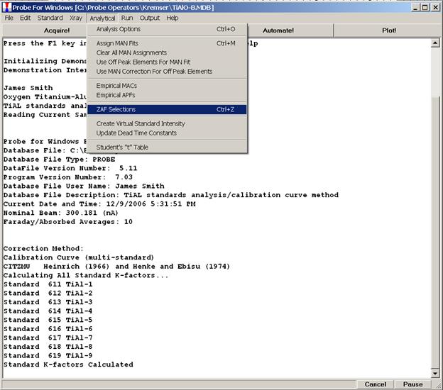
The Matrix Correction Methods window opens. Select the Calibration Curve (multi-standard) button for the Correction Method.
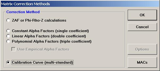
Click the OK button, returning to the main Probe for EPMA log window.
Next, the user will evaluate each of the three calibration curves. Open the Plot! window. Select all nine titanium-aluminide alloy standards to plot. Note, the check box for Force Black and White Print was selected. If the user wants to output and archive the graphed data, this option causes the printer to create a clean black and white print, without gray background (see discussion below). Select a Graph Type. Check the Average Only check box to use the average value of each standard sample.
Finally, plot O Elemental Percents versus O On Peak Counts (P+B).
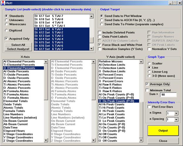
Click the Output button.
All of the selected standards are analyzed and reported in the main Probe for EPMA log window.
The Plot Graph Data window appears.
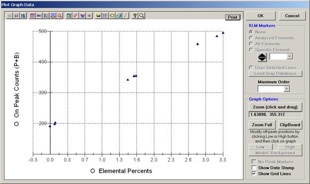
The Show Grid Lines check box has been marked to facilitate reading the percent and count values. This calibration curve may be printed out by clicking the Print button next to the OK button. If the user selects the Force Black and White Print check box in the Plot! window, then the corresponding output will be a black and white print, if not, then the printer will output the above gray background.
The user may evaluate the data using the Zoom Full capabilities (click and drag mouse over region of interest on graph) to expand the scaling. Here, in the center group, two data points clearly overlap. Placing the mouse cursor over any selected point on the graph returns the x and y values of that position (read above the Zoom Full button).
When finished, click the OK button to return to the Plot! window to next review the other calibration curves.
The output for aluminum is plotted similarly. Select the Al Elemental Percents versus Al On Peak Counts (P+B), (the counts per second determined on peak) and click the Output button in the Plot! window. This curve is viewed below.
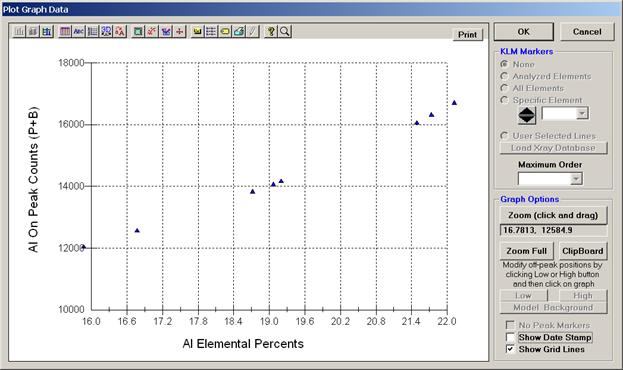
The graph may be modified by selecting any of the buttons across the top to enter the Graph Control module.
Graph Control (see tabs in display below) can be used to edit numerous graph parameters. Under the Trends tab, for instance, are the curve fitting options. Select Curve Fit under Statistical Lines and edit the Curve Fit Type and Order as required.
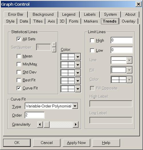
Click the Apply Now or OK button to see the changes in the Graph Data window.
The modified Plot Graph Data window returns. Here, a title, different, larger symbols, standard numbers and the second order polynomial curve have been added to the graph below.
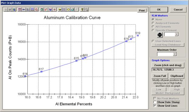
Upon creating the previous plots, the selected standards were analyzed, each of the nine standards were reported in the main Probe for EPMA log window along with the second order polynomial fit parameters.
The following output displays the log window output for one
of these: St 617 Set 5 TiAl-7 standard.
St  617 Set   5 TiAl-7
TakeOff = 52.5  KiloVolt = 15.0  Beam Current = 30.0  Beam Size =    1
(Magnification =        .)                    Beam Mode = Analog  Spot

Titanium aluminide 3.03 Oxygen
Number of Data Lines:  5               Number of 'Good' Data Lines:  5
First/Last Date-Time: 12/11/2000 04:03:01 PM to 12/11/2000 04:06:28 PM
WARNING- Using Calibration Curve Matrix Corrections

Average Total Oxygen:         .000     Average Total Weight%:  100.651
Average Calculated Oxygen:    .000     Average Atomic Number:   20.177
Average Excess Oxygen:        .000     Average Atomic Weight:   40.571

Results in Elemental Weight Percents

ELEM:       Al      Ti       O
BGDS:      LIN     LIN     LIN
TIME:    10.00   10.00   10.00

ELEM:       Al      Ti       O   SUM
   978  15.452  81.618   2.986 100.056
   979  15.680  81.966   3.114 100.761
   980  15.864  81.880   3.053 100.796
   981  15.788  81.957   3.000 100.744
   982  15.747  82.245   2.908 100.900

AVER:   15.706  81.933   3.012 100.651
SDEV:     .157    .224    .077
SERR:     .070    .100    .035
%RSD:      1.0      .3     2.6

PUBL:   15.730  81.240   3.030 100.000
%VAR:     -.15     .85    -.59
DIFF:    -.024    .693   -.018

UNCT:  13020.8 11807.2   329.4
UNBG:    215.5    29.2   116.0
PKBG:    61.44  406.68    3.84

FIT1:    .4671-363.4302  -.5152
FIT2:    .0013   .0712   .0098
FIT3:  .000000-.000003 .000003
DEV:       2.2      .9     7.1
The coefficients for the second order polynomial are listed last (Fit 1, Fit 2, Fit 3 and Dev). The three Fit terms represent the intercept, the slope and the second order curvature factor, respectively. The DEV term represents the total deviation (sum of the residuals) between the calculated curve and the original data. The smaller the number, the better here. The software prints a warning line if this correction method is active.
The analysis of unknown samples is straightforward. Create a new sample and collect the x-ray intensity data on the unknown. Select the Analyze! window and click Analyze.
An example is printed next.
Un   25 Sample 3-9 LowOx 0-30u 2u increments
TakeOff = 52.5  KiloVolt = 15.0  Beam Current = 30.0  Beam Size =    1
(Magnification =        .)                    Beam Mode = Analog  Spot
Number of Data Lines: 16               Number of 'Good' Data Lines: 16
First/Last Date-Time: 12/11/2000 01:27:41 PM to 12/11/2000 01:40:41 PM
WARNING- Using Calibration Curve Matrix Corrections

Average Total Oxygen:         .000     Average Total Weight%:   99.869
Average Calculated Oxygen:    .000     Average Atomic Number:   19.838
Average Excess Oxygen:        .000     Average Atomic Weight:   39.903

Results in Elemental Weight Percents

ELEM:       Al      Ti       O
BGDS:      LIN     LIN     LIN
TIME:    10.00   10.00   10.00

ELEM:       Al      Ti       O   SUM
   851  21.260  76.350   1.956  99.566
   852  21.236  76.469   2.003  99.708
   853  21.193  76.689   1.957  99.839
   854  21.128  76.174   1.941  99.244
   855  21.222  76.599   1.842  99.663
   856  21.120  76.425   1.755  99.300
   857  21.126  76.494   1.838  99.459
   858  21.125  77.135   1.767 100.027
   859  21.142  76.686   1.791  99.619
   860  21.153  76.835   1.796  99.784
   861  21.139  77.248   1.703 100.089
   862  21.256  77.439   1.685 100.379
   863  21.190  77.360   1.833 100.383
   864  21.216  77.503   1.779 100.499
   865  21.286  77.127   1.643 100.055
   866  21.264  77.541   1.482 100.287

AVER:   21.191  76.880   1.798  99.869
SDEV:     .058    .454    .133
SERR:     .015    .113    .033
%RSD:       .3      .6     7.4

UNCT:  18339.0 11021.6   222.4
UNBG:    218.2    26.6   113.8
PKBG:    85.05  417.09    2.96

FIT1:    .4718-363.4019  -.5152
FIT2:    .0013   .0712   .0098
FIT3:  .000000-.000003 .000003
DEV:       2.2      .9     7.1
The second order polynomial coefficients are always listed last (just above). Elements calculated by difference or stoichiometry can be calculated along with calibration curve corrected elements. And if both off-peak and MAN acquired data are present, Probe for EPMA will construct separate sets of calibration curves and fit a second order polynomial expression that is used in the iteration procedure to determine the concentration of the element.
The user may elect to run standards after completing unknown sample acquisition and then correct for any standard intensity drift. From the main Probe for EPMA log window select Analytical and then choose Analysis Options from the drop-down menu.
The Analysis Calculation Options window appears, remember to check that the Use Automatic Drift Correction on Standard Intensities check box is marked.
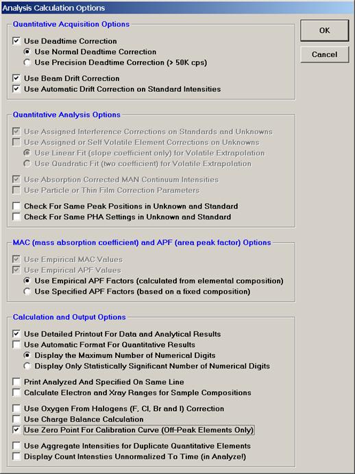
In some instances, it may be useful to add to the acquired data set a zero point (off-peak elements only) to improve the polynomial fit. To include a zero point, check the box (prior to analyzing the standards) labeled Use Zero Point For Calibration Curve (Off-Peak Elements Only). This choice is also found in the Analysis Calculation Options window.
Probe for EPMA gives the user two powerful methods for the correction of time-dependent intensities of elements in unknown samples. By time-dependent we mean a signal intensity that is varying with time in a smooth fashion, and due to the processes of element migration, volatilization, or any other process that results in a time-varying intensity. The term is used to indicate a generic process with perhaps incomplete knowledge of the details of the process involved (i.e., the term volatile is typically incorrect and cannot be confirmed by EPMA measurement alone). Each correction option provides a means to automatically correct data for the time-dependent loss of x-ray intensity due to continuous electron bombardment (heating damage/charge buildup) or carbon contamination that occurs during normal electron microprobe work. The time-dependent element extrapolation may be applied to any degradation (or enhancement) of the x-ray intensity over time. Elements most susceptible include sodium, potassium, perhaps sulfur and bound water. This correction is most useful for samples that are too small to utilize a defocused beam and also allows the operator to run higher than normal sample currents to improve analytical sensitivity.
Two different methods are available for time-dependent element corrections; the Self Calibration TDI Acquisition and the Assigned Calibration TDI Acquisition. Each will be documented.
In the Self Calibration TDI Acquisition method, the program acquires the on-peak count data for the time-dependent element during the normal sample acquisition process for the unknown sample. This method works well when samples to be analyzed have widely differing compositions as the calibration is determined with every sample acquisition.
Open Probe for EPMA, and proceed through the normal calibration and standardization routine. Check suitable standards for accuracy, these should not be time-dependent or beam sensitive.
Move to your first unknown sample. Open the New Sample window from the Acquire! window and create a new unknown sample.
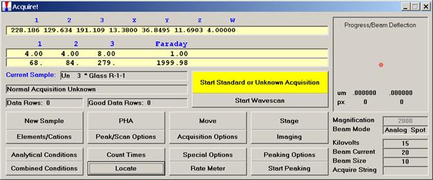
Click the Special Options button in the Acquire! window.
The TDI Calibration and Quick Wavescan Samples window opens. Select the Self Calibration TDI Acquisition option. The time-dependent element correction is only applied to the first element analyzed for on each spectrometer. Enter a number into the TDI Count Time Intervals text field (up to 50 intervals may be used). The program will use this interval number and the on-peak count time to create a calibration curve. In this example, Na is counted for 40 seconds on peak and with an interval of 10 entered, the program will automatically count ten 4 second intervals. Each element listed first on each spectrometer is treated in this way. The off peak counts are not affected.
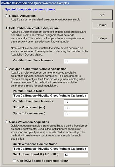
Click the OK button to return to the Acquire! window.
Click the Start Standard or Unknown Acquisition button to initiate count data collection on the unknown sample.
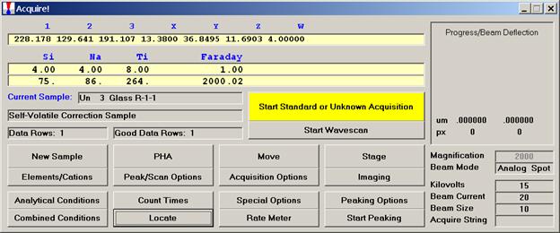
After collecting an unknown sample the user may display the time-dependent correction from the Analyze! window.
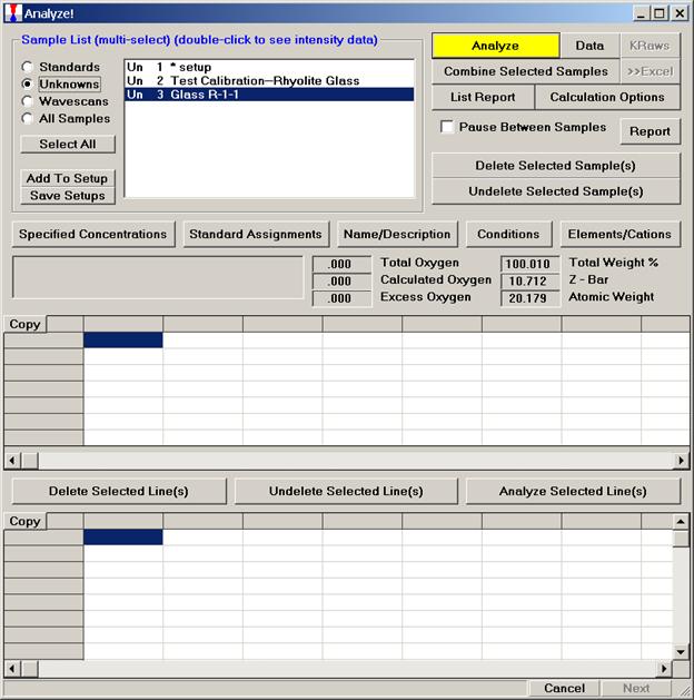
Click the Standard Assignments button.
The Standard and Interference Assignments window
opens.
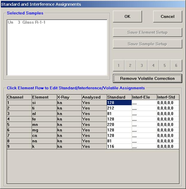
Select the element row (sodium in this example) to view the time-dependent calibration data.
The Assignment Properties window opens and lists all possible time-dependent element calibration samples.
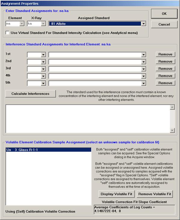
Highlight the appropriate TDI Element Calibration Sample Assignment sample and click the Display TDI Fit button.
The TDI (Self) Fit Plot window opens.
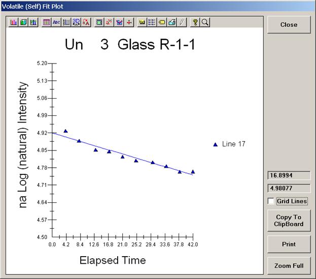
The drop in sodium count intensity with time appears to fit an exponential function (Nielson and Sigurdsson, 1981). A plot of the natural log of the intensity data versus time should yield a straight line relationship as seen above.
The extrapolation correction is quantitative in that the correction is based on a self calibration curve acquired during the run. The correction uses the actual elapsed time for all calculations. It is applied during the ZAF or Phi-Rho-Z iteration phase of the analysis to correct for changes in the matrix correction due to the extrapolation correction.
The next example will illustrate the Assigned Calibration TDI Acquisition method. Here, small rhyolitic glass inclusions of similar composition will be analyzed.
Start Probe for EPMA in the normal manner. Go through the calibration and standardization process, then check standards. Save the analysis routine as a sample setup. Next, create a separate sample setup with a subset of elements to which the time-dependent correction will be assigned, in this example silicon and sodium. Note time-dependent element calibration corrections can only be applied to elements that are the first element collected by each spectrometer.
Locate the sample to obtain the time-dependent element correction acquisition upon. This should be either the unknown sample or a material similar to the unknowns.
Click the Special Options button in the Acquire! window.
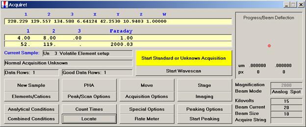
The TDI Calibration and Quick Wavescan Samples window opens. The default acquisition choice is Normal Acquisition.
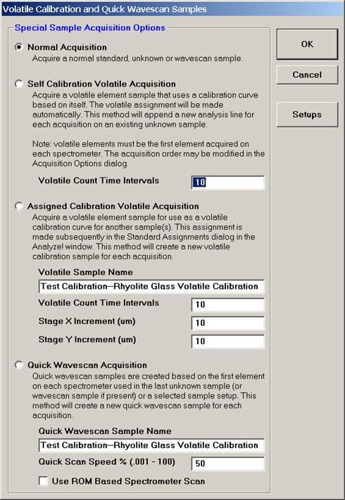
Click the Setups button in the TDI Calibration and Quick Wavescan Samples window, opening the Sample Setup Selection dialog box. Check that the appropriate volatile setup is active.
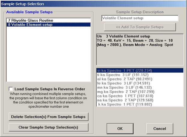
Click the OK button.
Select the Assigned Calibration TDI Acquisition method. Enter text into the Volatile Sample Name field. Edit the TDI Count Time Intervals (number of steps in the calibration line) and adjust the Stage X and Y Increment (um) values if required, resulting in the following window.
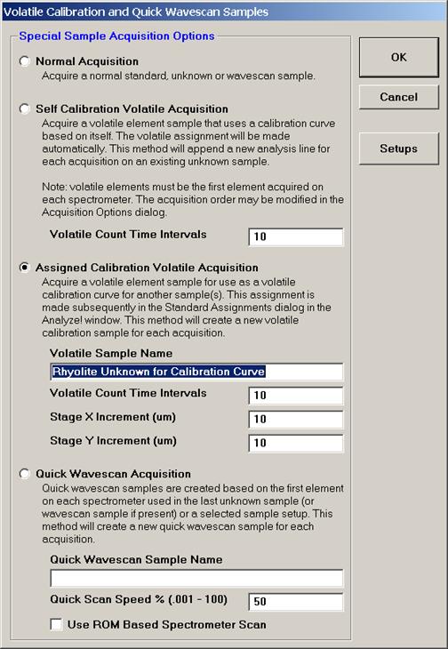
The time-dependent element effect will be calibrated precisely on the first unknown sample. One important assumption is that the time-dependent element behavior on the calibration sample is similar to all the unknowns to be analyzed. Therefore, because a consistent time-dependent correction is used, variation in composition represents real differences in composition (or volatilization) not precision of the analyses. Each element in the method (sample setup) will be acquired one element at a time. In this example, 10 time intervals are specified and the default on-peak count times for silicon and sodium are 20 and 40 respectively. Thus the calibration curve for each will be composed of 10 spots of 2 and 4 seconds each. The program will acquire each element in the sample (at a fresh spot) at a new stage position based on the X and Y increments specified to allow the time-dependent element effect to be calibrated precisely.
Click the OK button to return to the Acquire!
window.
The time-dependent sample acquisition will start automatically upon clicking the Start Standard or Unknown Acquisition button, using the sample name entered in the TDI Sample Name field.
The user may now collect unknown data points. REMEMBER to load in the appropriate sample setup AND under the Special Options button of the Acquire! window, click the Normal Acquisition button.
After collecting an unknown sample the user may assign the time-dependent correction from the Analyze! window.
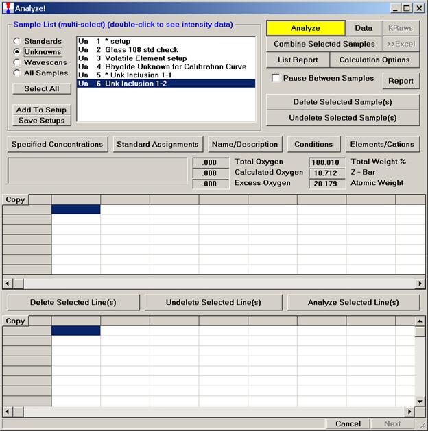
The time-dependent element calibration can be assigned to any element in a sample provided that it was acquired as the FIRST element on that spectrometer.
Click the Standard Assignments button. The Standard and Interference Assignments window opens.
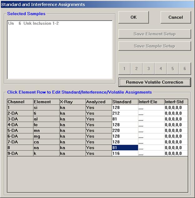
To evaluate the correction effect on sodium, click that element’s row to view and edit its’ time-dependent assignment.
The Assignment Properties window opens and lists all possible time-dependent element calibration samples.
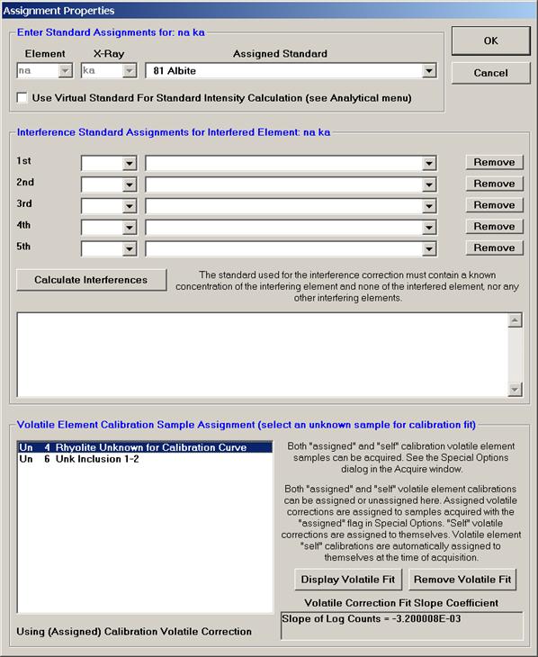
Highlight the appropriate TDI Element Calibration Sample Assignment sample and click the Display TDI Fit button.
The TDI (Assigned) Fit Plot window opens.
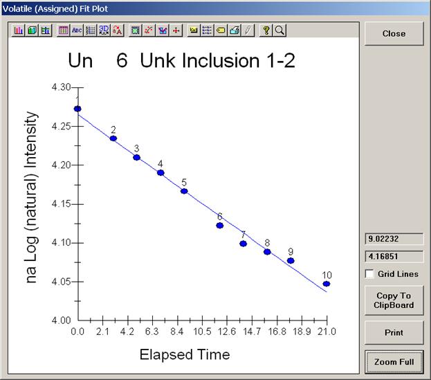
The drop in sodium count intensity with time appears to fit an exponential function (Nielson and Sigurdsson, 1981). A plot of the natural log of the intensity data versus time should yield a straight line relationship as seen above.
The extrapolation correction is quantitative in that the correction is based on a calibration curve acquired during the run. The correction uses the actual elapsed time for all calculations. It is applied during the ZAF or Phi-Rho-Z iteration phase of the analysis to correct for changes in the matrix correction due to the extrapolation correction.
Along with alkali loss, the operator may notice an increase in count intensity from the non-mobile elements (such as silicon and aluminum) in the sample. The possible enhancement with time may be corrected for as well.
Close the TDI (Assigned) Fit Plot window, returning to the Assignment Properties window. Click the OK button.
To evaluate the possible enhancement of intensity with time on silicon in the rhyolitic glass, click on the element row for silicon in the Standard and Interference Assignments window.
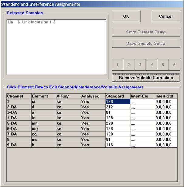
The Assignment Properties window opens. Again, highlight the appropriate TDI Element Calibration Sample Assignment sample and click the Display TDI Fit button.
The TDI (Assigned) Fit Plot window opens displaying the natural log of silicon x-ray intensity versus time. The enhancement is evident and maybe corrected for quantitatively.
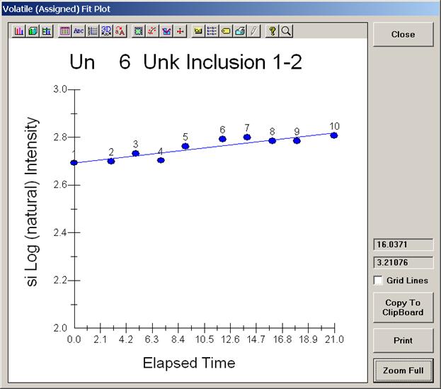
Return to the Analyze! window by clicking the Close button above.
Click the OK button of the Assignment Properties and the Standard and Interference Assignments windows, respectively.
Probe for EPMA permits the user to select a fully quantitative correction for spectral interferences (Donovan et al., 1993). The user can correct for up to four interfering elements per channel. The program requires that both the interfered and interfering elements be analyzed for. Further, an interference calibration standard must be acquired that contains a major concentration of the interfering element and none of the interfered element nor any other elements that interfere with the interfered element.
Most interferences between a pair of elements work in one direction. Consider a phase with high concentrations of manganese in the presence of the iron. Here the Mn Kβ line interferes with the Fe Kα analytical line. The reverse situation does not cause a problem, iron does not interfere with manganese. However, there are some cases where both elements interfere with each other! These dual interfering elements are extremely difficult to correctly quantify. Fortunately, Probe for EPMA can handle this situation because it’s quantitative interference correction is an iterated solution (see Donovan et al., 1993 for details).
The following example (analyzed at U.C. Berkeley by John Donovan) involves the dual interference of zinc and rhenium in a natural organo-metallic phase. Both lines interfere with each other (Zn Kβ and Re Lα) and both lines are used for quantitative analysis. Other elements analyzed for are cesium, iron, sulfur, and selenium. Oxygen, nitrogen, carbon and hydrogen are also in the samples. Each is listed in the Element/Cations window for use in the matrix correction routine but are not analyzed.
Solving these interferences requires the analyses of both rhenium and zinc and two interference standards. To correct for the interference on zinc, a standard that contains rhenium but no zinc is required. Likewise, to handle the interference on rhenium, a standard will be needed that contains zinc but no rhenium.
The procedure to specify interferences and the correction thereof was documented in the silicate chapter in the Users Guide to Getting Started manual, cogent details will briefly mentioned here.
To view the various interference assignments, click the Standard Assignment button in the Analyze! window.
The Standard and Interference Assignments window opens.
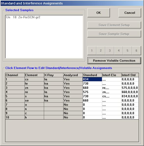
In John’s routine, Cs Lα is measured on the standard CsBr, likewise Fe Kα is done on a pyrite (FeS2) standard and the Se Kα line is measured on the ZnSe standard.
Zinc, rhenium and sulfur require additional discussion.
Highlighting the zinc element row opens the Assignment Properties window for that element. The user has the option to display all possible interferences based on the current set of analyzed and interfered elements. Clicking the Calculate Interference button displays these. The program calculates the interference based on a gaussian peak shape assuming a worst case scenario of 0.1% of the analyzed element and 100% of each of the other analyzed and possibly interfering elements.
As mentioned earlier and seen below, Re Lα interferes with the Zn Kα on the LIF crystal. To correct for this overlap, a standard with no zinc present (rhenium metal) is employed for the calculation.
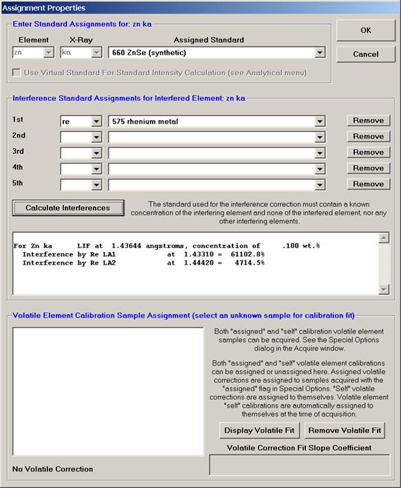
The Assignment Properties window for Re Lα is shown next. Here, Zn Kα interferes with the Re Lα x-ray position. To make the quantitative correction the standard ZnSe (with no rhenium) is used.
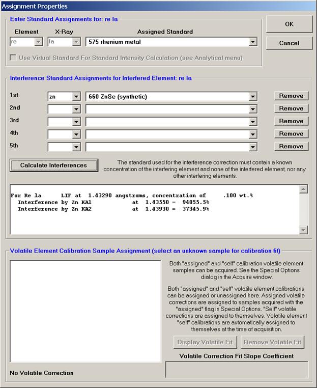
Finally, the Assignment Properties window for S Kα is displayed. In this unique mineral, Cs Lα overlaps with S Kβ. Therefore, a cesium standard without sulfur (CsBr) is also required to complete the spectral interference deconvolution!
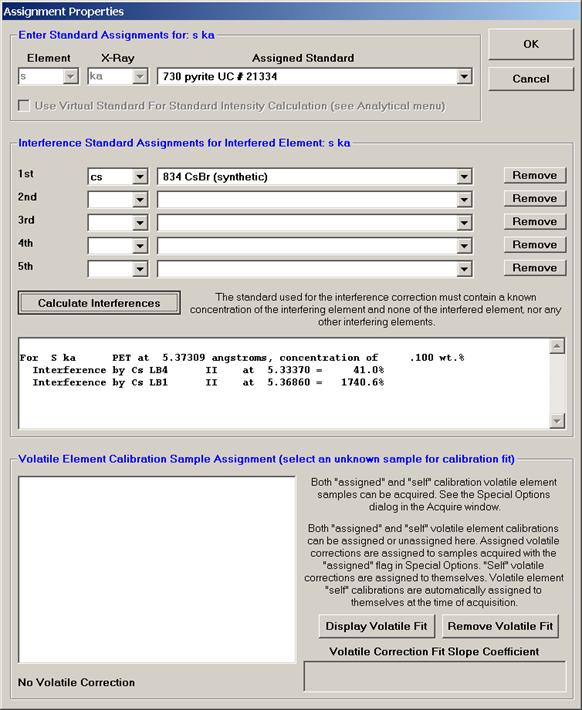
After setting up the parameters for the analysis session, calibration and standardization was accomplished, then several tiny and complex organometallic phases were probed for their chemistry.
The Analysis Calculation Options window allows the user to enable or disable the interference correction routine to view its effect on quantitative analysis results. This window is activated from the Analytical | Analysis Options menu in the main Probe for EPMA log window.
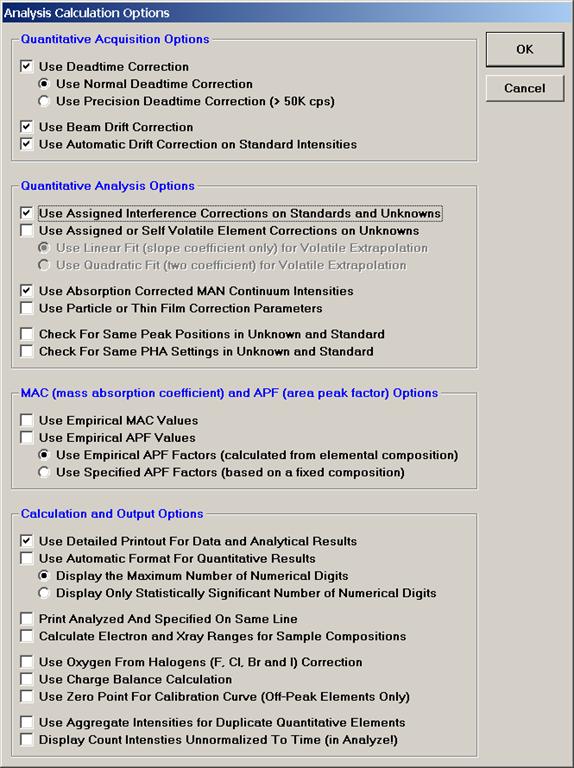
Data illustrating the power of the Probe for EPMA interference correction routine is shown below. The results are for a real unknown sample that has some variability and was rather small to analyze. The following unknown analysis is without any interference corrections.
Un   10 Zn-ReSCN gr2
TakeOff = 40.0  KiloVolt = 20.0  Beam Current = 20.0  Beam Size =    0
(Magnification =        .)                    Beam Mode = Analog  Spot
Number of Data Lines:  5               Number of 'Good' Data Lines:  3
First/Last Date-Time: 06/15/1998 04:39:29 PM to 06/15/1998 04:55:23 PM

Average Total Oxygen:         .000     Average Total Weight%:  122.912
Average Calculated Oxygen:    .000     Average Atomic Number:   53.080
Average Excess Oxygen:        .000     Average Atomic Weight:   54.153
Average ZAF Iteration:        4.00     Average Quant Iterate:     2.00


Results in Elemental Weight Percents

SPEC:        O       N       C       H
TYPE:     SPEC    SPEC    SPEC    SPEC

AVER:    1.900   5.000   4.200    .200
SDEV:     .000    .000    .000    .000

ELEM:       Cs      Fe      Zn      Re       S      Se
BGDS:      LIN     LIN     LIN     LIN     LIN     LIN
TIME:    10.00   10.00   10.00   10.00   10.00   10.00

ELEM:       Cs      Fe      Zn      Re       S      Se   SUM
    53    .000    .000  19.553  73.669  17.465    .000 121.988
    55    .000    .007  20.556  74.517  16.507    .000 122.886
    56    .000    .019  19.668  74.715  18.159    .000 123.862

AVER:     .000    .009  19.926  74.301  17.377    .000 122.912
SDEV:     .000    .010    .549    .556    .830    .000
SERR:     .000    .006    .317    .321    .479    .000
%RSD:       .1   113.3     2.8      .7     4.8      .1
STDS:      834     730     660     575     730     660

STKF:    .5978   .4297   .5001  1.0000   .4719   .5162
STCT:    627.1  3670.9  3712.9  3672.8  4423.1  1315.9

UNKF:    .0000   .0001   .2100   .6516   .0943   .0000
UNCT:     -2.7      .3  1559.2  2393.0   884.3    -3.2
UNBG:     11.6    28.0    67.3    61.5     6.6    64.0

ZCOR:   1.2016   .9276   .9487  1.1404  1.8421  1.0254
KRAW:   -.0043   .0001   .4199   .6516   .1999  -.0024
PKBG:      .77    1.01   24.18   40.00  135.89     .95

Results Based on 6 Atoms of re

SPEC:        O       N       C       H
TYPE:     SPEC    SPEC    SPEC    SPEC

AVER:    1.786   5.368   5.258   2.983
SDEV:     .013    .040    .039    .022

ELEM:       Cs      Fe      Zn      Re       S      Se   SUM
    53    .000    .000   4.536   6.000   8.260    .000  34.323
    55    .000    .002   4.714   6.000   7.718    .000  33.784
    56    .000    .005   4.499   6.000   8.468    .000  34.281

AVER:     .000    .002   4.583   6.000   8.149    .000  34.129
SDEV:     .000    .003    .115    .000    .387    .000
SERR:     .000    .002    .067    .000    .224    .000
%RSD:       .8   113.2     2.5      .0     4.8      .8
The user immediately realizes that there is a problem since
the unknown sums to a total of 123%.
The following is the same unknown but with the iterated
interference software applied.
Un   10 Zn-ReSCN gr2
TakeOff = 40.0  KiloVolt = 20.0  Beam Current = 20.0  Beam Size =    0
(Magnification =        .)                    Beam Mode = Analog  Spot
Number of Data Lines:  5               Number of 'Good' Data Lines:  3
First/Last Date-Time: 06/15/1998 04:39:29 PM to 06/15/1998 04:55:23 PM

Average Total Oxygen:         .000     Average Total Weight%:  101.367
Average Calculated Oxygen:    .000     Average Atomic Number:   54.332
Average Excess Oxygen:        .000     Average Atomic Weight:   50.124
Average ZAF Iteration:        4.00     Average Quant Iterate:    13.00


Results in Elemental Weight Percents

SPEC:        O       N       C       H
TYPE:     SPEC    SPEC    SPEC    SPEC

AVER:    1.900   5.000   4.200    .200
SDEV:     .000    .000    .000    .000

ELEM:       Cs      Fe      Zn      Re       S      Se
BGDS:      LIN     LIN     LIN     LIN     LIN     LIN
TIME:    10.00   10.00   10.00   10.00   10.00   10.00

ELEM:       Cs      Fe      Zn      Re       S      Se   SUM
    53    .000    .000   6.237  65.851  17.508    .000 100.896
    55    .000    .007   7.365  65.342  16.513    .000 100.527
    56    .000    .020   6.100  67.048  18.210    .000 102.678

AVER:     .000    .009   6.568  66.080  17.410    .000 101.367
SDEV:     .000    .010    .694    .876    .853    .000
SERR:     .000    .006    .401    .506    .492    .000
%RSD:       .1   113.3    10.6     1.3     4.9      .0
STDS:      834     730     660     575     730     660

STKF:    .5978   .4297   .5001  1.0000   .4719   .5162
STCT:    627.1  3670.9  3712.9  3672.8  4423.1  1315.9

UNKF:    .0000   .0001   .0691   .5781   .0943   .0000
UNCT:     -2.7      .3   512.7  2123.2   884.3    -3.2
UNBG:     11.6    28.0    67.3    61.5     6.6    64.0

ZCOR:   1.2162   .9395   .9511  1.1431  1.8455  1.0235
KRAW:   -.0043   .0001   .1381   .5781   .1999  -.0024
PKBG:      .77    1.01    8.61   35.59  135.89     .95
INT%:      .00     .00  -67.17  -11.27     .00     .00

Results Based on 6 Atoms of re

SPEC:        O       N       C       H
TYPE:     SPEC    SPEC    SPEC    SPEC

AVER:    2.008   6.036   5.913   3.355
SDEV:     .026    .080    .078    .044

ELEM:       Cs      Fe      Zn      Re       S      Se   SUM
    53    .000    .000   1.619   6.000   9.264    .000  34.252
    55    .000    .002   1.926   6.000   8.805    .000  34.239
    56    .000    .006   1.555   6.000   9.463    .000  34.083

AVER:     .000    .003   1.700   6.000   9.177    .000  34.191
SDEV:     .000    .003    .199    .000    .337    .000
SERR:     .000    .002    .115    .000    .195    .000
%RSD:      1.2   112.3    11.7      .0     3.7     1.3
The total now is acceptable, slightly over 100%.
Finally to demonstrate with standard samples (of known
composition), both rhenium metal and the ZnSe standard will be reproduced
without the benefit of the interference correction.
St  575 Set   1 rhenium metal
TakeOff = 40.0  KiloVolt = 20.0  Beam Current = 20.0  Beam Size =    0
(Magnification =        .)                    Beam Mode = Analog  Spot
Number of Data Lines:  5               Number of 'Good' Data Lines:  5
First/Last Date-Time: 06/15/1998 01:40:14 PM to 06/15/1998 01:48:18 PM

Average Total Oxygen:         .000     Average Total Weight%:  124.489
Average Calculated Oxygen:    .000     Average Atomic Number:   67.420
Average Excess Oxygen:        .000     Average Atomic Weight:  142.028
Average ZAF Iteration:        3.00     Average Quant Iterate:     2.00

Results in Elemental Weight Percents

ELEM:       Cs      Fe      Zn      Re       S      Se
BGDS:      LIN     LIN     LIN     LIN     LIN     LIN
TIME:    10.00   10.00   10.00   10.00   10.00   10.00

ELEM:       Cs      Fe      Zn      Re       S      Se   SUM
     1    .000    .000  21.083 103.240    .022    .000 124.344
     2    .161    .005  20.061 102.988    .008    .000 123.223
     3    .000    .000  21.644 103.274    .000    .176 125.093
     4    .000    .023  21.565 103.834    .000    .156 125.578
     5    .000    .000  19.873 104.122    .000    .213 124.207

AVER:     .000    .000  20.845 103.492    .000    .109 124.489
SDEV:     .072    .010    .833    .469    .009    .102
SERR:     .032    .004    .372    .210    .004    .045
%RSD:    223.6   177.2     4.0      .5   159.1    93.2

PUBL:    n.a.    n.a.    n.a.  100.000   n.a.    n.a.  100.000
%VAR:      .00     .00     .00    3.49     .00     .00
DIFF:     .000    .000    .000   3.492    .000    .000
STDS:      834     730     660     575     730     660

STKF:    .5978   .4297   .5001  1.0000   .4719   .5162
STCT:    628.0  3665.4  3726.7  3679.3  4367.5  1316.2

UNKF:    .0003   .0001   .2405  1.0000   .0000   .0012
UNCT:       .0    -1.1  1792.2  3679.3     -.4     1.8
UNBG:     11.6    41.9    95.5    93.5     8.4    93.4

ZCOR:   1.2008   .8713   .8667  1.0349  2.1623   .9212
KRAW:    .0000  -.0003   .4809  1.0000  -.0001   .0013
PKBG:     1.00     .97   19.77   40.37     .95    1.02


St  660 Set   1 ZnSe (synthetic)
TakeOff = 40.0  KiloVolt = 20.0  Beam Current = 20.0  Beam Size =    0
(Magnification =        .)                    Beam Mode = Analog  Spot
Number of Data Lines:  5               Number of 'Good' Data Lines:  5
First/Last Date-Time: 06/15/1998 01:50:41 PM to 06/15/1998 01:58:46 PM

Average Total Oxygen:         .000     Average Total Weight%:  151.911
Average Calculated Oxygen:    .000     Average Atomic Number:   47.924
Average Excess Oxygen:        .000     Average Atomic Weight:   92.977
Average ZAF Iteration:        3.00     Average Quant Iterate:     2.00

Results in Elemental Weight Percents

ELEM:       Cs      Fe      Zn      Re       S      Se
BGDS:      LIN     LIN     LIN     LIN     LIN     LIN
TIME:    10.00   10.00   10.00   10.00   10.00   10.00

ELEM:       Cs      Fe      Zn      Re       S      Se   SUM
     6    .000    .000  44.441  55.414    .019  51.417 151.290
     7    .000    .014  44.022  56.029    .036  51.668 151.768
     8    .000    .000  44.551  56.249    .035  51.099 151.934
     9    .000    .015  44.700  56.069    .037  50.974 151.795
    10    .000    .000  45.281  56.025    .052  51.409 152.767

AVER:     .000    .000  44.599  55.957    .036  51.314 151.911
SDEV:     .000    .008    .457    .317    .012    .277
SERR:     .000    .003    .204    .142    .005    .124
%RSD:       .0   137.1     1.0      .6    33.5      .5

PUBL:    n.a.    n.a.   45.290   n.a.    n.a.   54.710 100.000
%VAR:      .00     .00   -1.53     .00     .00   -6.21
DIFF:     .000    .000   -.691    .000    .000  -3.396
STDS:      834     730     660     575     730     660

STKF:    .5978   .4297   .5001  1.0000   .4719   .5162
STCT:    628.0  3665.4  3726.6  3679.0  4367.5  1316.2

UNKF:    .0000   .0001   .5002   .5193   .0002   .5162
UNCT:    -23.1    -1.4  3726.7  1910.6     1.7  1316.2
UNBG:     29.3    23.0    48.3    47.7     5.6    47.5

ZCOR:   1.1332   .8826   .8917  1.0775  1.9149   .9940
KRAW:   -.0367  -.0004  1.0000   .5193   .0004  1.0000
PKBG:      .21     .95   78.18   41.17    1.31   28.85
The rhenium standard displays an apparent rhenium concentration of 103% and a zinc total of an additional 20%. The ZnSe is even more interesting in that the total is approaching 152% with 44% zinc, 56% rhenium and 51% selenium. The true composition is 45% zinc, and 55% selenium with no rhenium! The normal matrix correction comes close with respect to both zinc and selenium abundances but also reports a whopping 56% rhenium concentration.
Below, both standards are rerun with the interference corrections applied.
St  575 Set   1 rhenium metal
TakeOff = 40.0  KiloVolt = 20.0  Beam Current = 20.0  Beam Size =    0
(Magnification =        .)                    Beam Mode = Analog  Spot
Number of Data Lines:  5               Number of 'Good' Data Lines:  5
First/Last Date-Time: 06/15/1998 01:40:14 PM to 06/15/1998 01:48:18 PM

Average Total Oxygen:         .000     Average Total Weight%:  100.138
Average Calculated Oxygen:    .000     Average Atomic Number:   74.736
Average Excess Oxygen:        .000     Average Atomic Weight:  184.273
Average ZAF Iteration:        2.00     Average Quant Iterate:    13.80

Results in Elemental Weight Percents

ELEM:       Cs      Fe      Zn      Re       S      Se
BGDS:      LIN     LIN     LIN     LIN     LIN     LIN
TIME:    10.00   10.00   10.00   10.00   10.00   10.00

ELEM:       Cs      Fe      Zn      Re       S      Se   SUM
     1    .000    .000    .375  99.332    .023    .000  99.730
     2    .164    .005    .000  99.625    .007    .000  99.801
     3    .000    .000   1.096  98.532    .000    .168  99.796
     4    .000    .023    .847  99.364    .000    .149 100.383
     5    .000    .000    .000 100.776    .000    .203 100.979

AVER:     .000    .000    .463  99.526    .000    .104 100.138
SDEV:     .074    .010    .496    .810    .010    .097
SERR:     .033    .004    .222    .362    .004    .043
%RSD:    223.6   177.2   107.0      .8   164.6    93.2

PUBL:    n.a.    n.a.    n.a.  100.000   n.a.    n.a.  100.000
%VAR:      .00     .00     .00    -.47     .00     .00
DIFF:     .000    .000    .000   -.474    .000    .000
STDS:      834     730     660     575     730     660

STKF:    .5978   .4297   .5001  1.0000   .4719   .5162
STCT:    628.0  3665.4  3726.7  3679.3  4367.5  1316.2

UNKF:    .0003   .0001   .0055   .9942   .0000   .0012
UNCT:       .0    -1.1    10.3  3657.8     -.4     1.8
UNBG:     11.6    41.9    95.5    93.5     8.4    93.4

ZCOR:   1.2302   .8692   .8409  1.0011  2.3003   .8800
KRAW:    .0000  -.0003   .0028   .9942  -.0001   .0013
PKBG:     1.00     .97    1.11   40.14     .95    1.02
INT%:      .00     .00  -99.57    -.59   -2.86     .00

St  660 Set   1 ZnSe (synthetic)
TakeOff = 40.0  KiloVolt = 20.0  Beam Current = 20.0  Beam Size =    0
(Magnification =        .)                    Beam Mode = Analog  Spot
Number of Data Lines:  5               Number of 'Good' Data Lines:  5
First/Last Date-Time: 06/15/1998 01:50:41 PM to 06/15/1998 01:58:46 PM

Average Total Oxygen:         .000     Average Total Weight%:  100.261
Average Calculated Oxygen:    .000     Average Atomic Number:   32.317
Average Excess Oxygen:        .000     Average Atomic Weight:   72.276
Average ZAF Iteration:        3.00     Average Quant Iterate:    14.80

Results in Elemental Weight Percents

ELEM:       Cs      Fe      Zn      Re       S      Se
BGDS:      LIN     LIN     LIN     LIN     LIN     LIN
TIME:    10.00   10.00   10.00   10.00   10.00   10.00

ELEM:       Cs      Fe      Zn      Re       S      Se   SUM
     6    .000    .000  45.120    .000    .017  54.799  99.936
     7    .000    .014  44.451   1.080    .032  54.982 100.559
     8    .000    .000  45.152    .477    .032  54.459 100.120
     9    .000    .015  45.415    .000    .033  54.368  99.831
    10    .000    .000  46.003    .000    .047  54.807 100.857

AVER:     .000    .000  45.228    .311    .032  54.683 100.261
SDEV:     .000    .008    .560    .477    .011    .259
SERR:     .000    .003    .251    .213    .005    .116
%RSD:       .0   137.1     1.2   153.1    33.5      .5

PUBL:    n.a.    n.a.   45.290   n.a.    n.a.   54.710 100.000
%VAR:      .00     .00    -.14     .00     .00    -.05
DIFF:     .000    .000   -.062    .000    .000   -.027
STDS:      834     730     660     575     730     660

STKF:    .5978   .4297   .5001  1.0000   .4719   .5162
STCT:    628.0  3665.4  3726.6  3679.0  4367.5  1316.2

UNKF:    .0000   .0001   .4995   .0028   .0002   .5162
UNCT:    -23.1    -1.4  3721.5     2.3     1.7  1316.2
UNBG:     29.3    23.0    48.3    47.7     5.6    47.5

ZCOR:   1.0893   .8842   .9055  1.1054  1.7229  1.0593
KRAW:   -.0367  -.0004   .9986   .0006   .0004  1.0000
PKBG:      .21     .95   78.08    1.05    1.31   28.85
INT%:      .00     .00    -.14  -99.88     .00     .00
Now, the apparent zinc in the rhenium metal standard is gone and the average total sums correctly near 100%. The ZnSe standard is perfect, matching the published standard composition for both zinc and selenium, and effectively removing all of the apparent 56% rhenium.
Quantitative analysis of light elements (beryllium to fluorine) is difficult to do correctly with the electron microprobe. Numerous issues impede the analysis of light elements (see Appendix B in the User’s Guide and Reference documentation as well as Goldstein et al., 1992 for further discussion). A few brief comments will be made here, as an introduction to this section.
Typically, for x-ray analysis in this energy range (0.1 to 0.7 keV), a large absorption correction is necessary. This large correction in conjunction with the fact that the mass absorption coefficients for the low energy x-rays are very large and not very well known (see Appendix C of the User’s Guide and Reference documentation) place a severe demand on the established ZAF and Phi-Rho-Z models for light element matrix corrections. Some reduction in this large x-ray absorption factor is possible by analyzing at higher take-off angles and at lower acceleration voltages. The former aids by shortening the path length for absorption in the sample while the latter involves a decrease in the electron beam penetration so that x-rays are generated closer to the surface and can escape to be detected.
Low count rates for these light elements are often found. This is due to the low fluorescent yields from the Kα x-ray lines and the inefficient nature of WDS counting systems. Count rates can be increased by increasing the beam current substantially but this may then lead to deadtime problems for metal lines that interfere with the light element lines of interest. The use of new layered dispersive element (LDE) synthetic multi-layer crystals with large d-spacings can also improve light element peak count rates.
There is also a strong possibility of interferences from higher order metal lines such as titanium, chromium, manganese, iron, nickel, zirconium, niobium, and molybdenum with the light element lines. These interferences are often severe for minor and trace level measurements. It is critical to eliminate peak overlaps and understand the background intensity around the light element peak position in both the sample and standard. The new LDE multi-layer crystals also help here by strongly suppressing these higher order reflections.
Finally, chemical bonding effects can result in wavelength shifts, increases or decreases in the relative intensities of various lines and alteration of the shape of the analytical line. These effects are most significant for the lightest (lowest energy) elements. Polarization phenomena and crystallographic orientation may also cause variations in peak shape and intensity especially for boron. Therefore, to measure the intensity of the light elements, one measures the integral intensity (area) under the characteristic peak rather than just the peak intensity.
Bastin and Heijliers (1984, 1991) pioneered the area-peak factor (APF) analysis method. The APF is defined as the ratio between the integral intensity (area) k-ratio from the sample and the standard and the peak intensity k-ratio from the same sample and the standard. This factor is only valid for a given compound with respect to a given standard and a specific spectrometer setup. These integral measurements can be made by scanning the spectrometer in small steps across the characteristic peak with the wavescan feature in Probe for EPMA. After acquiring the peak shape profiles for a primary standard and a number of secondary standards and correcting for the background and removal of interfering peaks, the APF can be calculated as:

Where :
 is the integrated intensity of the secondary standard
 is the peak intensity of the primary standard
 is the peak intensity of the secondary standard
 is the integrated intensity of the primary standard
After an APF has been determined, future measurements of that compound can be accomplished by measuring only the peak intensity in the sample and standard. Then, multiplication of the peak k-ratio with the appropriate APF will yield the correct integral k-ratio.
Probe for EPMA allows the user to select an APF correction for use in correcting x-ray intensities for peak shift and shape changes between the standard and the multi-element unknown. This is critical when the user is analyzing the Kα lines of the light elements (boron, carbon, nitrogen and oxygen). This correction may also be of use for other elements such as S Kα that also exhibits peak shift and shape changes when comparing sulfate and sulfide peaks.
The power of this correction will be documented in the analysis of oxygen using several simple oxide standards. Open a new Probe for EPMA run. Here oxygen Kα will be analyzed using MgO as the calibration standard. The spectrometer is equipped with a standard P-10 gas flow counter and a LDE (59.8Å) W/Si reflecting crystal. The other two elements to be determined are magnesium on MgO and silicon on SiO2 . Peak the three elements and acquire standard samples for each.
Create a new unknown sample and collect data on the SiO2 standard. Analyze the sample from the Analyze! window.

A low total for the analysis is found. The nominal composition for the SiO2 standard is silicon: 46.74 and oxygen: 53.26. Here, the discrepancy in the total rests primarily with the oxygen concentration. The low oxygen concentration is independent of the matrix correction (and mass absorption coefficient) and can only be corrected for by using the appropriate APFs.
Select Analytical | Analysis Options from the main Probe for EPMA log window to open the Analysis Calculation Options window. Click the Use Empirical APF Values check box to activate this option.
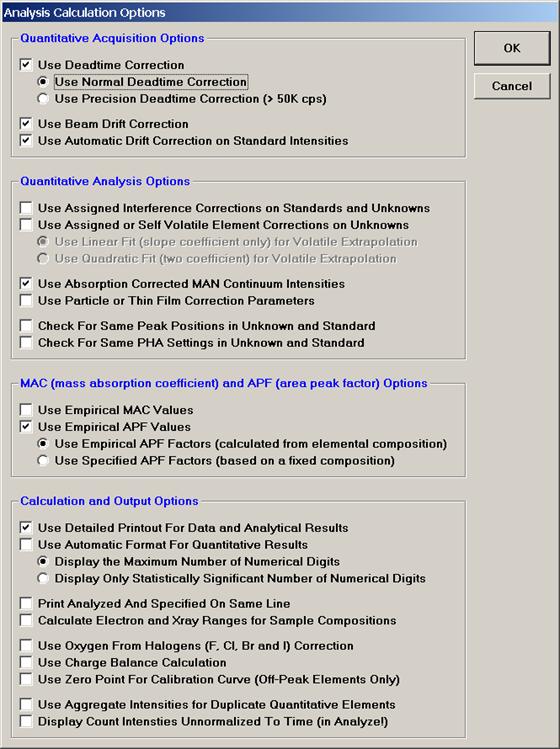
Click the OK button.
Next, select Analytical | Empirical APFs from the main Probe for EPMA log window to open the Add Empirical APFs (area peak factors) to Run window.
Find the appropriate correction. Two choices are given for oxygen in the presence of SiO2, Bastin’s value of 1.04440 using Fe2O3 as the calibration standard and Donovan’s correction factor of 1.070 when using MgO as the calibration standard. Although the values seen in the text field below are relative to Fe2O3, the APF for MgO relative to Fe2O3 is also 1.000, which means that these correction factors apply equally well relative to MgO. Hence, the use of MgO as the calibration standard.
The APF correction values are defined in the EMPAPF.DAT file in the Probe for EPMA directory. The file contains some 80 values that may or may not be applicable, depending on the analyzing crystals and standards available. It is strongly recommended that the user measure the integral intensities and peak intensities and calculate the APFs for your particular spectrometer setup. And if necessary, edit the EMPAPR.DAT file using any ASCII text editor such as NotePad to insert their own measurements. See the User’s Guide and Reference documentation for editing format and details.
Click the Add To Run >> button to place the
selected empirical APF into the run.
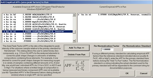
Click the OK button.
Re-analyze the unknown SiO2 sample. The total is now closer to 100% and a more reasonable oxygen concentration is calculated.
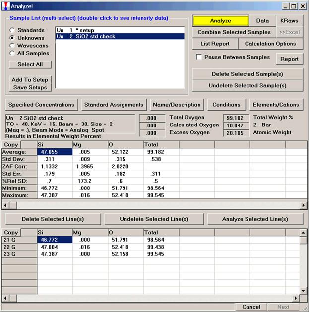
The APF values selected or entered are always measured relative to some standard sample. For example, if measuring oxygen Kα and using either MgO or Fe2O3 as the primary standard for oxygen, then any oxygen Kα APF values used must be those measured relative to either MgO or Fe2O3. For the same reason, if using APF values for a particular light element and the user decides to re-assign the standard for that element, the APF values for that element must also be re-normalized to reflect the standard re-assignment.
Thus, it is most efficient to always use the same standard
for each light element analyzed. Typically (in order to utilize the APF values in the supplied EMPAPF.DAT file) these will be:
- Oxygen : MgO or Fe2O3
- Nitrogen : AlN
- Carbon : Fe3C
- Boron : B metal
The APF correction in Probe for EPMA will allow the user
to enter empirical APF values in each run. The user may enter one or more APF
factors for each emitting element although they are generally applied to soft
x-ray lines. The APF for each absorber will be summed according to it's weight
fraction in the composition and applied to the emitting element counts during
the ZAF or Phi-Rho-Z iteration.
Bastin G.F., and Heijliers H.J.M., (1984) Quantitative Electron-Probe Microanalysis of Carbon in Binary Carbides., Microbeam Analysis (Editors: A.D. Romig, Jr. and J.I. Goldstein) pp 291-294.
Bastin G.F., and Heijliers H.J.M., (1991) Quantitative Electron-Probe Microanalysis of Ultra-Light Elements (Boron-Oxygen)., Electron Probe Quantitation (Editors: K.F.J. Heinrich and D.E. Newbury), New York: Plenum Press pp 145-161.
Deer W.A., Howie R.A., and Zussman J., (1992) An introduction to The Rock-Forming Minerals, Second Edition, New York: Wiley.
Donovan J.J., Snyder D.A., and Rivers M.L., (1993) An Improved Interference Correction for Trace Element Analysis. Microbeam Analysis 2 23-28.
Goldstein J.I., Newbury D.E., Echlin P., Joy D.C., Romig A.D. Jr, Lyman C.E., Fiori C., and Lifshin E., (1992) Scanning Electron Microscopy and X-Ray Microanalysis, Second Edition, New York: Plenum.
Nielsen C.H., and Sigurdsson H., (1981) Quantitative methods for electron microprobe analysis of sodium in natural and synthetic glasses. Am. Mineral., 66 547-552.
Reed S.J.B., (1993) Electron-Microprobe Analysis, Second Edition, New York: Wiley.
Scott V.D., Love G.,and Reed S.J.B. (1995)
Quantitative Electron-Probe Microanalysis, Second Edition, London: Ellis Horwood.
Willis J.P., (1993) Course on Theory and Practice of XRF Spectrometry, University of Western Ontario, Department of Geology, Course Notes.
Startwin Program
Launch the Startwin program.
This is the main window of the Startwin Program:
This is the Count Acquisition window:
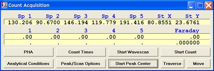
The Startwin program can be used for the following utility functions:
- Replicate measurement of probe current
- Replicate measurement of spectrometers at peak positions, with or without background measurement
- Spectrometer peaking
- A spectrometer alignment scan (z-axis scan) where all spectrometers are peaked over a vertical scan through the microprobe optical focus position
- PHA measurements including detector bias, gain, and SCA scans for all spectrometers
These capabilities are outlined in the following sections.
See the Startwin help documentation for further information.
Beam and Detector Stability
Testing beam (drift) stability is an important step prior to acquiring any quantitative data. The following step-by-step procedure illustrates how to monitor and plot beam current with time. On JEOL microprobes the FARADAY module may also be run for measurement of the beam (see the User’s Guide and Reference documentation for further details).
From the STARTWIN log window, select Modes from the menu bar and click on Cycle Counters from the menu choices. The Measure Faraday menu should also be selected.
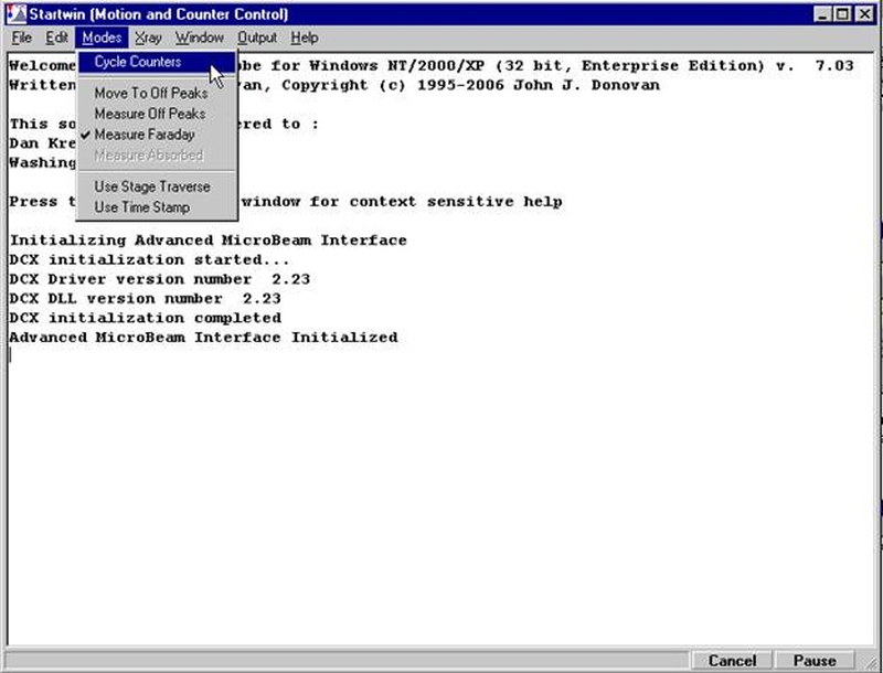
Next, click the Count Times button in the Count Acquisition window.
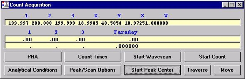
This opens the Count Times dialog box. Choose an On Peak and Cycle Time count time. The On Peak time is the time the scalers will count and the Cycle Time is the interval of time between successive measurements. Thus, the sum of both numbers is the time between measurements of the beam. Finally, disable the beam drift correction, confirm that the Use Beam Drift Correction box is unchecked.
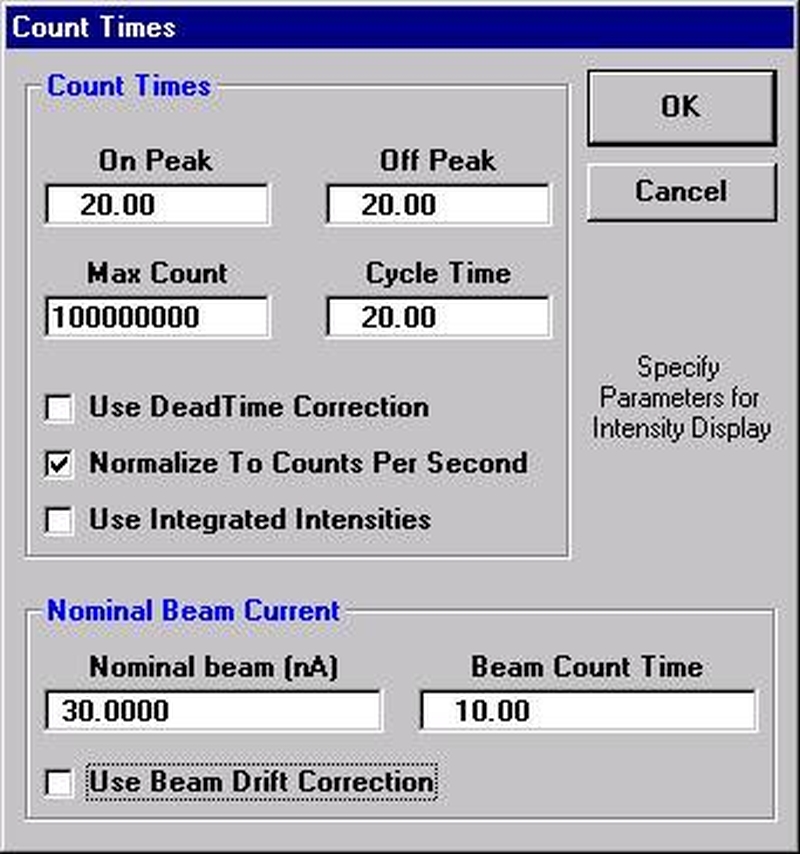
Click the OK button returning to the Count Acquisition window.
Click the Start Count button to initiate a continuous cycle of beam current measurements. In this example, a twenty second scaler count will be done followed by a twenty-second countdown and then a Faraday current measurement. This process repeats until the user cancels the loop.

When the user has acquired a suitable number of beam current measurements, click the Cancel button in the Automation Status bar located at the bottom right side of the STARTWIN log window to stop the acquisition cycle.
The STARTWIN log window will contain the beam current data acquired so far (in this example, reported in nanoamps). The other three columns represent counts in counts per second acquired by each spectrometer with the beam blanked (essentially detector/electronics noise).
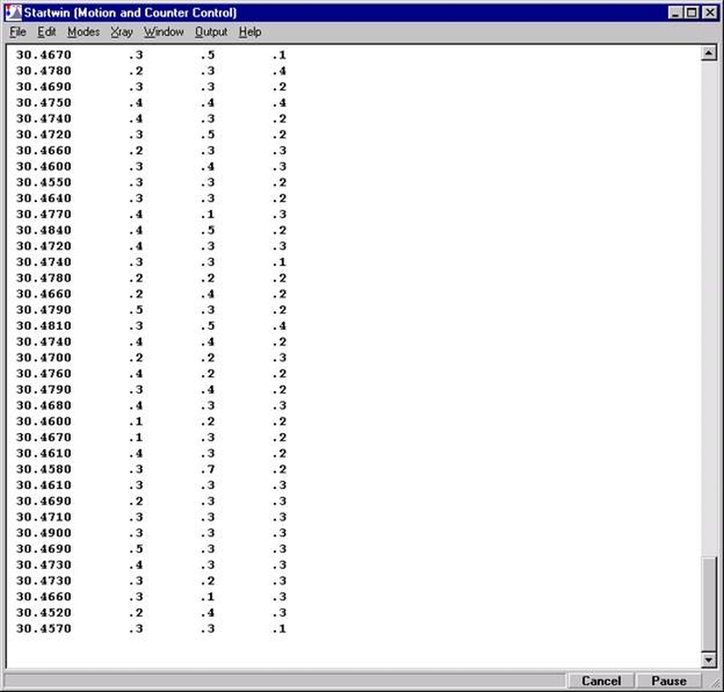
Evaluating the trend between beam current and time may best be viewed in graphical format rather than in looking at a long series of numbers. Use the mouse to select the data set to graph. Then, select Output from the menu bar and click Plot Count Data (Selected in Log Window) from the drop-down menu choices.
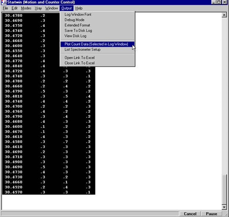
This opens the Display Data window.
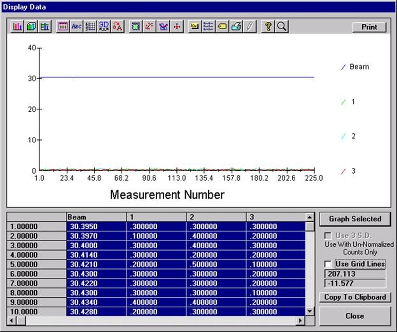
While all data columns were selected by the mouse operation previously, the user may plot a single column of data by clicking the column label of the desired data and then clicking the Graph Selected button.
Below, Beam Counts versus Measurement Number (time) are graphed and the overall beam stability with time may be judged. Here, the beam measurements fluxuate in the second decimal place (between 30.40 and 30.49).
The numeric value of any point on the graph maybe read by placing the mouse cursor over the data point and viewing it’s value in the two windows directly above the Close button (bottom right).
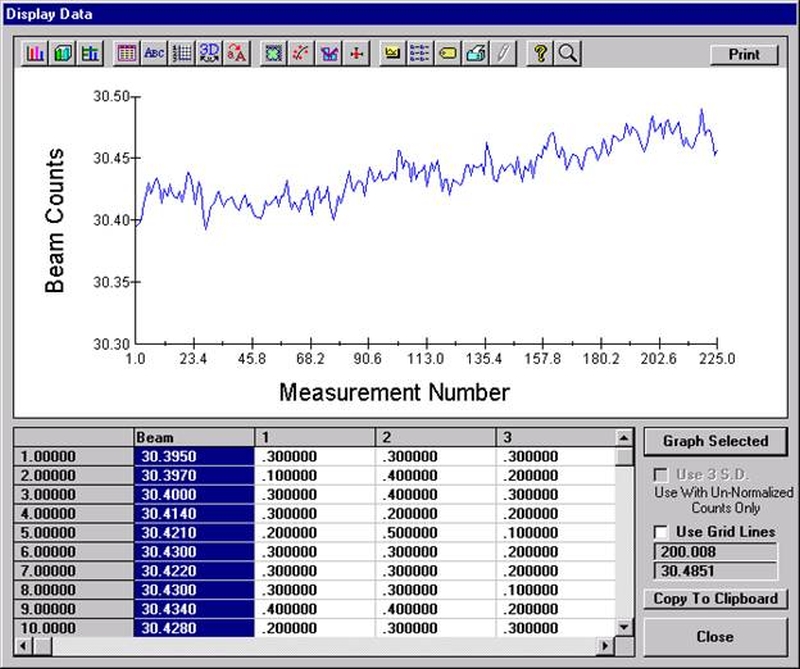
Click the Close button to return to the STARTWIN log window.
Determination of WDS Spectrometer Alignment
It is important to confirm that all wavelength-dispersive spectrometers (WDS) on the microprobe are individually aligned with respect to the Rowland circle, and further that all WDS are mutually aligned so that all Rowland circles are coincident at the sample focus position. Two components of alignment are necessary:
- A baseplate alignment moves the Rowland circle vertically so that the maximum X-ray intensity is observed at the optical focus z-axis position of the sample. This alignment is typically performed using an X-ray peak that is close to the low spectrometer limit and is therefore sensitive to vertical positioning of the Rowland circle.
- A crystal alignment is an adjustment of the diffracting crystal position so that the crystal is tangential to the Rowland circle. This adjustment is made by adjusting the angular positioning mechanism of the crystal, and is typically made at an X-ray peak position that is intermediate along the spectrometer travel.
- The complete alignment of the WDS thus ensures that the sample (at optical focus z-axis position), diffracting crystal, and X-ray detector are all mutually on the Rowland circle. The spectrometer mechanism must further maintain this alignment as the WDS is driven along the entire spectrometer range. It is necessary to check the alignment using several X-ray peaks to confirm this alignment throughout the range.
- The mutual alignment of all WDS on the microprobe is demonstrated by simultaneous measurement of the relative X-ray intensity, or k-ratio of an element with all WDS spectrometers. For example, all WDS simultaneously measure the intensity of Cu Kα on a pure Cu standard, then a second measurement is made on (for example) a NIST CuAu standard. The k-ratios measured on all WDS must agree within counting statistics, otherwise a misalignment is indicated.
Determination of WDS Spectrometer Deadtime
Currently done using Excel spreadsheet with Probe for EPMA Remote Automation Interface.
Determination of Pulse Height Analysis Parameters
Pulse Height Analysis
It is important to properly discriminate between the X-ray pulses produced by the sample and baseline noise which is also produced by the detector system. Remember that unlike an EDS pulse processing system, the WDS pulse processing electronics do not have digital electronics that automatically process the pulses and ignore the noise pulses. The WDS system requires that you properly set the detector voltage (hereafter referred to as the bias), gain, baseline, and window for X-ray counting. The procedure established on the Caltech JEOL 733 microprobe was to vary the detector bias in order to produce a 4V voltage pulse on a single-channel analyzer (SCA) plot. This was to reduce the detector deadtime dependence on X-ray energy. More practically, this approach allows the analyst to use a consistent baseline and window setting for all elements, but does require that specific detector bias values are used for the element being analyzed.
The proper PHA settings for WDS analysis require that the effective gain is sufficient to cleanly separate the X-ray pulses from the baseline noise of the detector system. All WDS counting systems are operated at a detector voltage, typically referred to as the bias, which is typically 1500-1900 volts, and results in the detector operating in the proportional counter range, where a photon produces a signal that is proportional to the X-ray energy.
The effect of increasing the detector bias is to increase the effective resolution of the X-ray pulse from the baseline noise, so that on an SCA plot the X-ray pulse moves to a higher voltage value. The effect of increasing the detector gain is to also increase the resolution and also moves the pulse to a higher SCA voltage. In practice, there are equivalent sets of bias and gain settings that should result in identical counting performance as measured by P/B and total count rate. Given the sets of equivalent bias and gain values, it is prudent to use a higher gain coupled with a lower detector bias in order to maximize the life of the detector. This implicitly assumes that modern counting systems do not exhibit increased noise at higher gain settings, which appears to be the case. You should demonstrate to your own satisfaction that these relationships are observed on your system.
Two different approaches are used for JEOL and Cameca microprobes which result in similar discrimination of pulses from baseline noise. On the JEOL microprobe, the detector gain is chosen from integer values of (typically) 16x, 32x, 64x, or 128x, and the bias is adjusted relative to the chosen gain value in order to achieve the proper PHA settings.
On the Cameca microprobe, the gain is continuously variable and the procedure is to choose a detector bias and adjust the gain value again in order to achieve the proper PHA settings. Experience with WDS counting systems has revealed that there is a dependance of the deadtime of the counting electronics on X-ray energy, which can be minimized by always applying the same effective gain to the X-rays being measured. This is the reason for adjusting the bias and gain in order to produce a consistent single channel analyzer (SCA) plot of the observed voltage distribution returned from the counting electronics. On a JEOL microprobe the bias and gain are set to obtain a ~4V SCA pulse, and on a Cameca microprobe the bias and gain are set to obtain a ~2.5V SCA pulse distribution. These relationships are summarized below:
JEOL Microprobe PHA Method
For a given spectrometer, generally two gain values can be used that cover all X-ray energies for the crystals on that spectrometer:
- For TAP use 64x and 128x gain
- For PET use 64x and 128x gain on sealed detectors, 16x and 32x on flow detectors.
- For LiF use 32x and 64x gain (but for higher energy K-lines may need to use 16x gain and for lower energy lines may need to use 128x gain). Note similar issue with LiF on flow counter as for PET.
- For all light element analysis using LDE crystals, use 128x gain
- Select the gain-bias pair with higher gain and lower bias. Perform a bias scan using a ~3.8v baseline and 0.2v window. The maximum intensity on the bias scan will result in a ~4V pulse position on an SCA scan
- Note the following issues with bias/gain measurements. First, all measurements should be made at no higher than ~20K cps in order to minimize gain shifts due to count rate effects. Secondly, aging or electronic degradation of the detector itself or in combination with possible problems in the counting electronics can result in bias/gain values that do not agree with these general settings. Disagreement with other comparable spectrometers on the microprobe and/or excessively high bias values may indicate problems with the detector.
Cameca Microprobe PHA Method
- For all analyzing crystals, use "typical" bias value and perform gain scans using ~2.1V baseline and 0.2V window in order to obtain a ~2.25V pulse position on an SCA scan.
- This will require sets of bias values for high energy vs. low energy X-ray lines.
After the peak position has been determined, it is important to verify that the Pulse Height Analysis (PHA) settings are correct for this element. The spectrometer peak position can be determined with PHA settings that are only approximately correct since the peak intensity is usually obvious. The reverse approach is not practical as adjusting the PHA settings requires that the spectrometer is already tuned to the peak position.
Move Motors window showing current spectrometer positions before move operation:
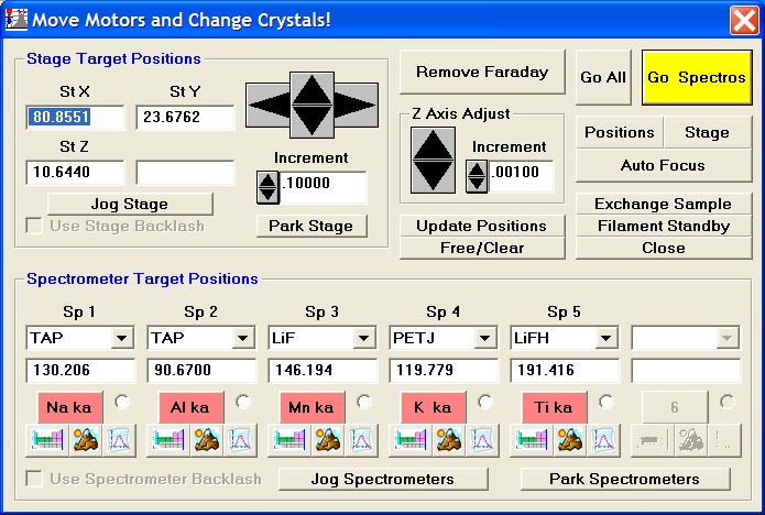
Spectrometer 3 is selected for Cu Kα using the LiF crystal:
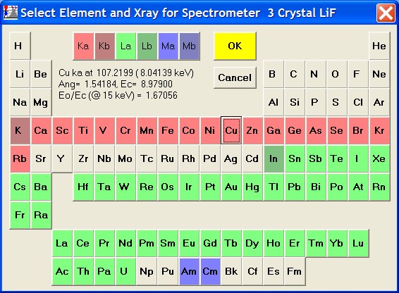
Move Motors window showing spectrometer positions after move operation (drive to Cu peaks all spectrometers):
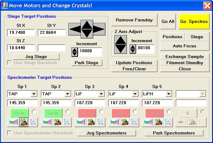
Peak/Scan Options selected and display of peak positions before update:
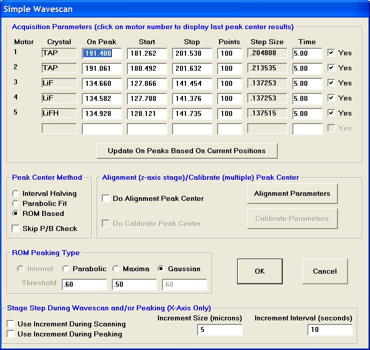
Peak/Scan Options display of peak positions after update (spectrometer positions have been updated):
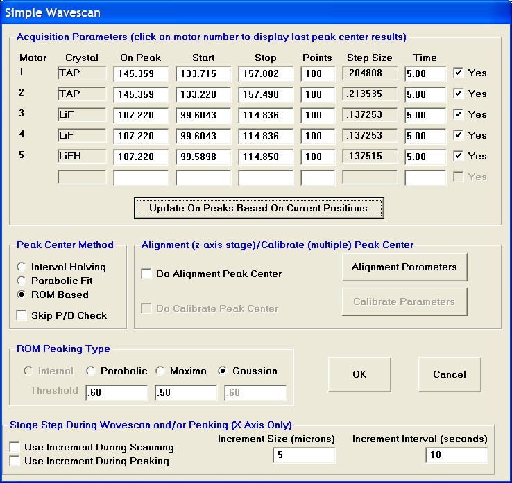
All spectrometers have been peaked and peaking results are displayed:
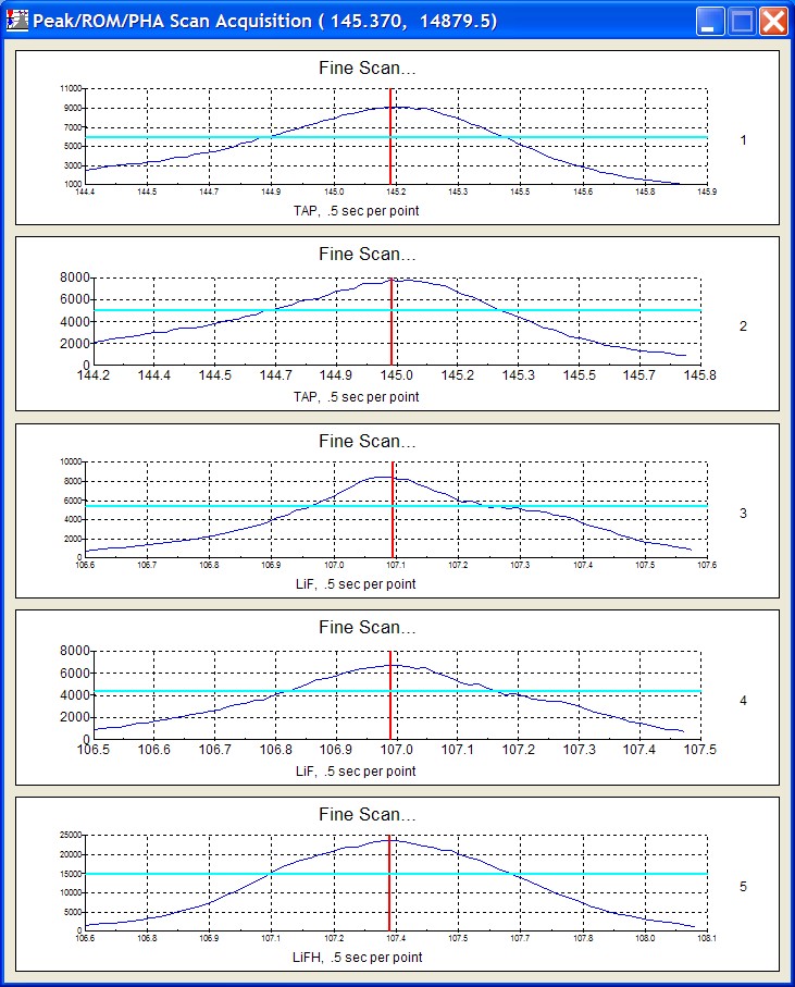
PHA button is clicked to open Pulse Height Analysis Parameters Window:
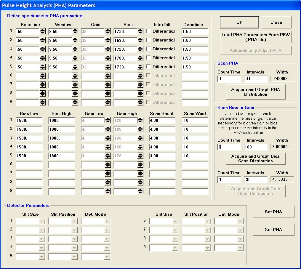
A Bias Scan is initiated and the results are shown for all spectrometers:
NEED PLOT
Summary of bias scan for all spectrometers on Cu at 32x gain:
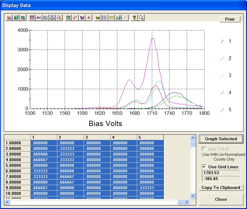
Summary of bias scan for spectrometer 5 on Cu at 32x gain:
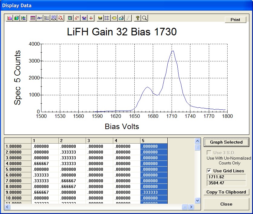
SCA scan acquired on all spectrometers using 32x gain and bias values determined from bias scan. Note that now the correct bias has been used and all SCA scans show a pulse at ~4V:
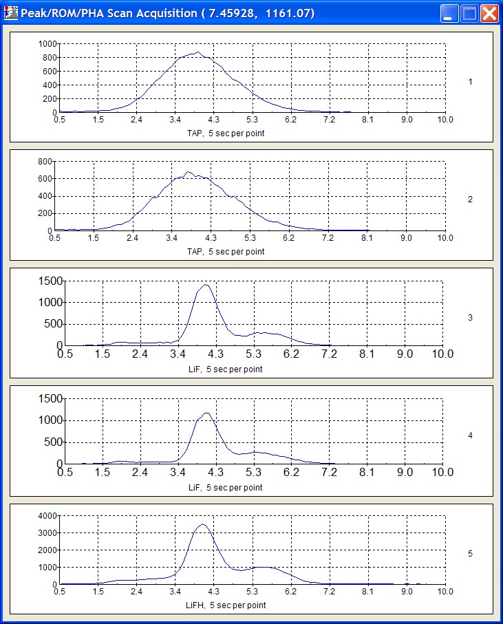
Summary of SCA scan acquired on all spectrometers using 32x gain and bias values determined from bias scan. Note the broad pulse distribution of Cu Lα compared to the sharper distribution for Cu Kα. Light element and low energy X-ray pulses will generally be smeared out on an SCA plot, and the determination of the baseline voltage setting is more important:
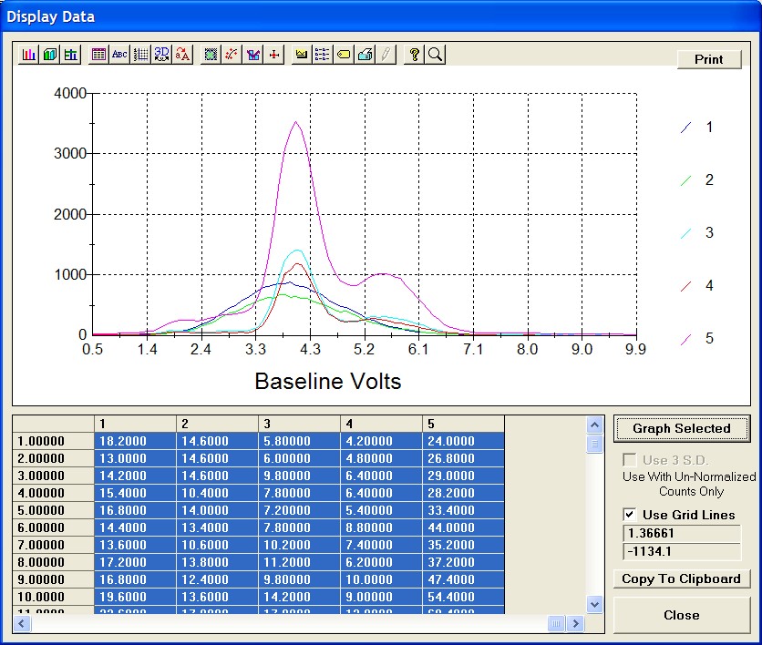
Long count SCA scan acquired on all spectrometers using 32x gain and bias values determined from bias scan. Note the broad distribution of pulses, this is the reason for using integral count mode:
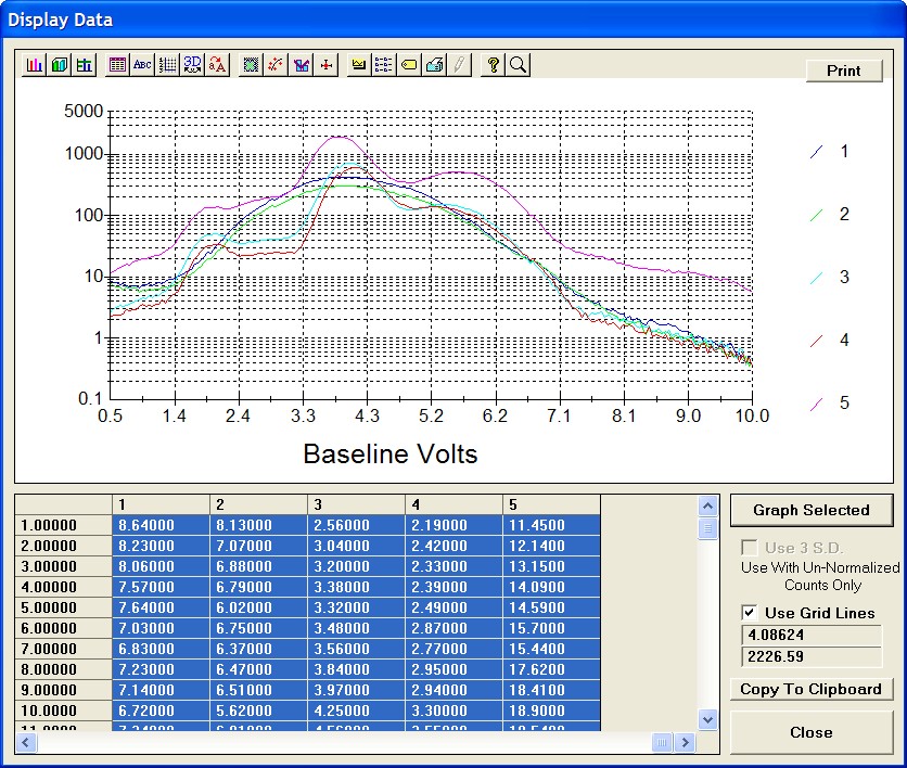
PHA Parameters: Gain Scans (Cameca)
This section awaits PHA scans obtained on Cameca instruments...by Cameca operators...you know who you are.
For Cameca instruments one uses a fixed bias value for all elements measured on that detector, and uses a specific gain value for each element since the gain can be varied over a significant range. So for Cameca setups one obtains gain scans that are specific to an element x-ray energy in order to obtain a PHA scan with a pulse at the desired voltage.
Because the Cameca uses P-10 Ar-methane gas for all counters, it is necessary to perform PHA scans on standards containing K, Ca, Sc, Ti, etc. for K-lines, and on In, Sn, Sb, etc. for L-lines. These PHA plots will reveal the presence of the Ar escape peak which must be either included or excluded as necessary for measurement.
PHA Parameters: SCA Scans
The term PHA stands for "pulse height analysis" and the term SCA stands for "single channel analyzer" (the terms PHA and SCA seem to be used interchangeably). EDS counting systems have a sophisticated pulse processing system using digital electronics that are capable of very high throughput and discrimination of X-ray pulses from one another and from background noise. Because WDS detector counting systems do not have the sophisticated pulse discrimination capabilities that EDS systems have, it is necessary for the operator to select the detector bias and/or gain as well as the baseline and window for pulse processing. As has been discussed, a bias scan is used on JEOL instruments to determine the bias that is used for a specific gain value in order to obtain an SCA scan with the pulse at ~4V. For the Cameca a gain scan is used for a specific bias in order to obtain an SCA scan at ~2V.
SCA Scans on P-10 Flow Counters
All Cameca detectors and the JEOL flow-proportional counters use P-10 Ar-methane gas mixture. For measurements using these flow-proportional counters, it is necessary to perform SCA scans to determine the proper baseline and window settings for routine measurement. The baseline setting is to eliminate baseline detector/electronics noise from measurement. A detector that exhibits a significant count rate with the electron beam turned off is likely passing noise counts due to a baseline that is too low. It is recommended to use the integral window setting rather than differential mode in order to accomodate pulse pileup at higher count rates. The importance of PHA energy discrimination has diminished since modern WDS spectrometers have excellent X-ray resolution so that PHA overlaps are not typically observed. While any higher order X-ray pulse that is diffracted at the same spectrometer position as the line of interest requires PHA discimination via specific baseline and window settings, this is not typical.
It is critically important to determine the baseline setting especially for light elements as the X-ray pulse energy is similar to that of the baseline noise. SCA scans should be acquired for light element measurement for each analytical session
SCA Scans on P-10 Flow Counters -- Ar Escape Peaks
X-rays that have an energy just above the Ar Kα excitation energy (K-edge) will fluoresce an Ar Kα X-ray which escapes from the detector since it is not strongly absorbed by the Ar detector gas. The Ar excitation energy and X-rays which produce an Ar escape peak are:
- Ar excitation energy is 3.2 keV. X-rays with energies close to and above this energy will be strongly absorbed and fluoresce an Ar Kα X-ray.
- K-lines producing an Ar escape peak: K (3.313 keV), Ca (3.691 keV), Sc (4.09 keV), Ti (4.51 keV), Cr (5.41 keV) (and on a Cameca, Mn, Fe, etc.).
- L-lines producing an Ar escape peak: In (3.287 keV), Sn (3.444 keV), Sb (3.605 keV), Te (3.769 keV), etc.
- No M alpha lines have sufficient energy to produce an Ar escape peak.
- The escape peak for K Kα is at lowest voltage with progressive movement of the escape peak into the main pulse distribution for higher energy X-rays.
- This means that a higher baseline is required for elements producing an escape peak at low voltage.
- On a JEOL flow-proportional spectrometer using a PET crystal, Cr Kα is the most energetic K-line that can be practically accessed, and Sm Lα is the most energetic L-line that can be accessed.
- On Cameca instruments one can observe the Ar escape peaks as discussed here but also for Mn, Fe, etc. since all spectrometers use P-10 flow counters.
Note that for X-rays having energies less than the Ar excitation energy, no escape peak is generated (e.g., for all K-lines up to Ar Kα, all L-lines up to Cd Lα, and all Mα lines). Also, for X-rays with energies significantly above the Ar excitation energy the escape peak is buried in the main pulse distribution and is not observed.
The best policy is to understand the pulse distribution and to either include or exclude the escape peak by proper selection of the PHA baseline.
Example SCA Scans Using P-10 Flow Counter on a JEOL 8200 with Ar Escape Peaks
The following plots show SCA plots for the K-lines of K, Ca, Sc, Ti, V, and Cr, and were obtained by placing the spectrometer at the peak position, acquiring a bias scan in order to determine the bias necessary to obtain a ~4V pulse on a SCA scan, then acquiring an SCA scan. In each case a typical microprobe standard was used (microcline for K, wollastonite for Ca, etc.). All data were acquired at 15kV and varying probe currents as required for necessary count rates. The SCA scans were obtained at 0.1 V steps with 5 sec per step.
All SCA scans superimposed to show progressive shift in Ar escape peak position with increasing X-ray energy.
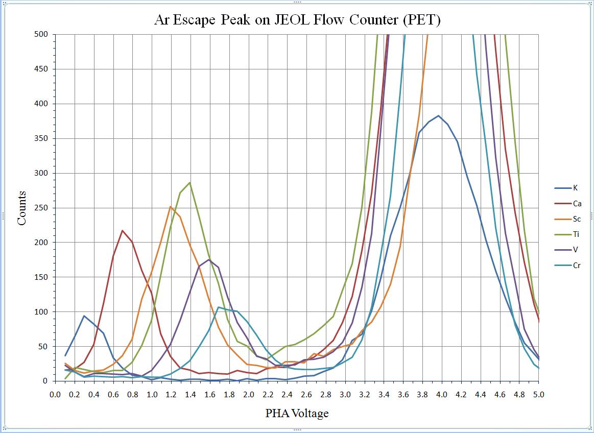
SCA scan for K (JEOL P-10 counter, PET crystal, microcline)
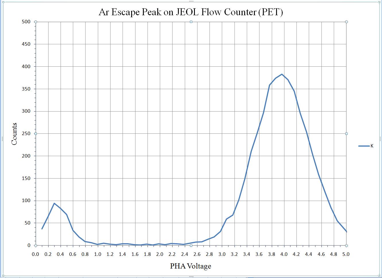
SCA scan for Ca (JEOL P-10 counter, PET crystal, wollastonite)
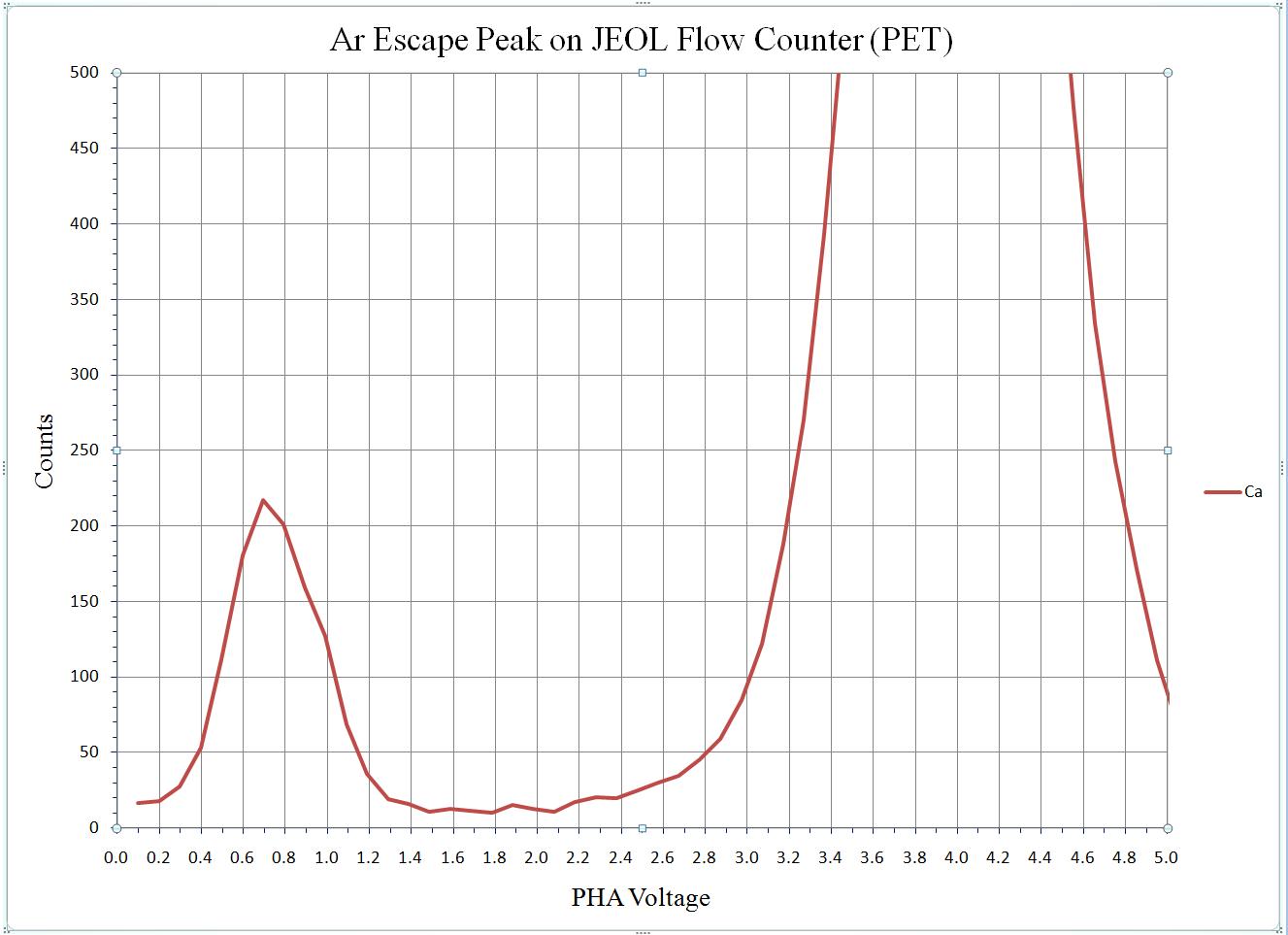
SCA scan for Sc (JEOL P-10 counter, PET crystal, Sc metal)
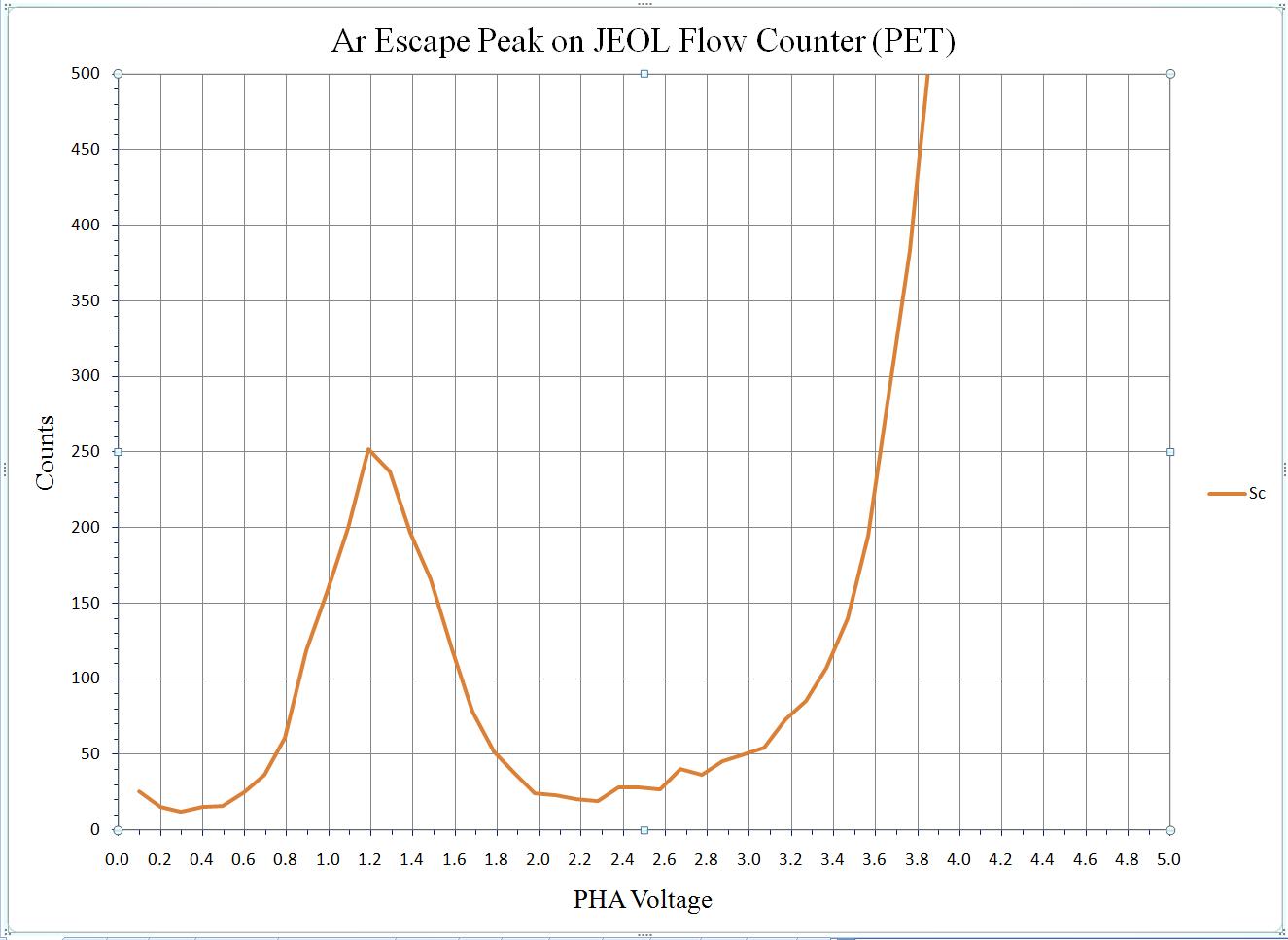
SCA scan for Ti (JEOL P-10 counter, PET crystal, TiO2)
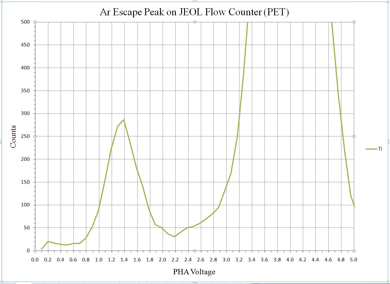
SCA scan for V (JEOL P-10 counter, PET crystal, V metal)
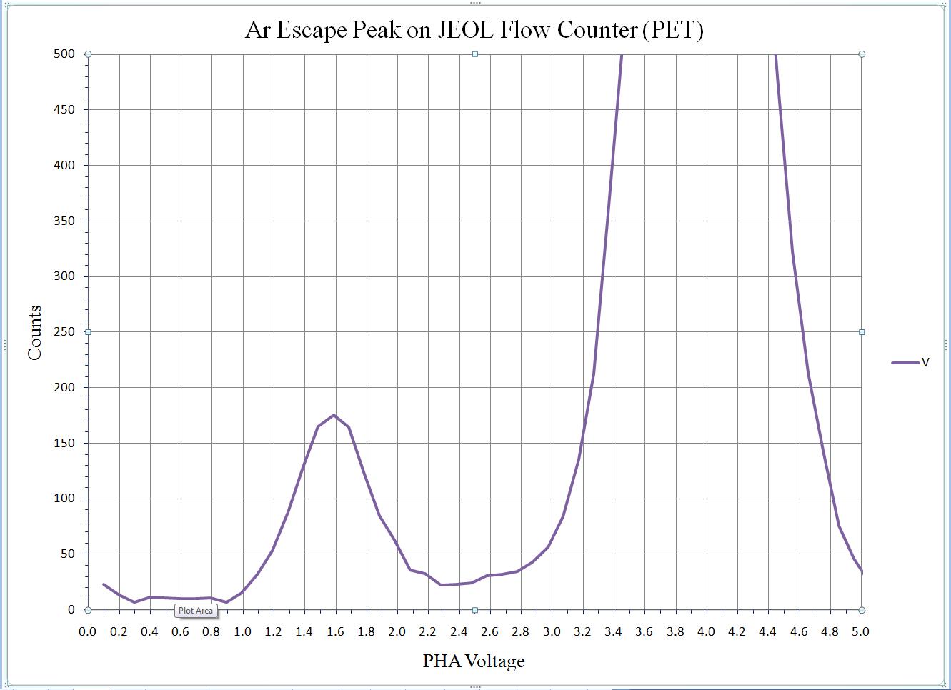
SCA scan for Cr (JEOL P-10 counter, PET crystal, Cr2O3)
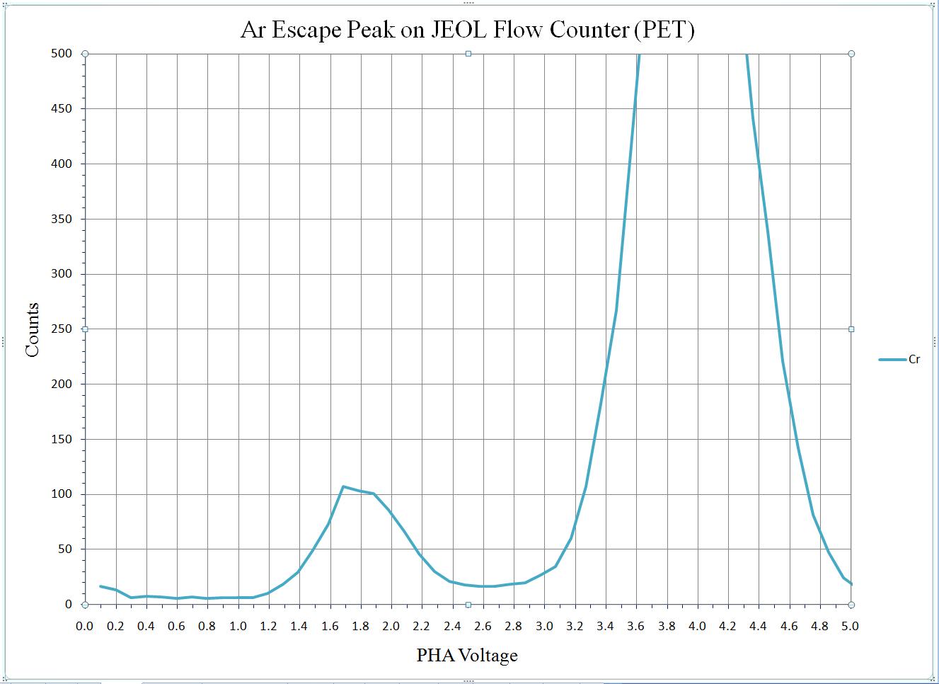
SCA Scans on JEOL Sealed Counters -- Xe Escape Peaks
JEOL instruments have sealed Xe detectors that are used with PET and LiF crystals for the analysis of more energetic X-rays. In the same fashion as for Ar escape peaks, X-rays that have an energy just above the Xe Lα excitation energy (LIII-edge) will fluoresce a Xe Lα X-ray which escapes from the detector since it is not absorbed by the Xe detector gas. Note, however, that the size of the Xe escape peak is smaller than the Ar escape peak due to the higher Z of Xe and inherent stronger attenuation of X-rays as a result. The Xe excitation energy and X-rays which produce an Xe escape peak are:
- Xe Lα excitation energy is 4.782 keV, this is the Xe LIII edge energy. X-rays with energies close to and above this energy will be strongly absorbed and fluoresce an Xe Lα X-ray.
- K-lines producing a Xe escape peak: V (4.952 keV), Cr (5.414 keV), Mn (5.898 keV), Fe (6.403 keV), etc.
- L-lines producing a Xe escape peak: Ce (4.840 keV), Pr (5.034 keV), Nd (5.230 keV), (Pm), Sm (5.636 keV), etc.
- No M alpha lines have sufficient energy to produce a Xe escape peak.
- The escape peak for V Kα is at lowest voltage with progressive movement of the escape peak into the main pulse distribution for higher energy X-rays.
- This means that a higher baseline is required for elements producing an escape peak at low voltage.
Again, the best policy is to understand the pulse distribution and to either include or exclude the escape peak by proper selection of the PHA baseline.
Example SCA Scans Using Sealed Xe Counter on a JEOL 8200 with Xe Escape Peaks
The following plots show SCA scans for K-lines of V, Cr, Mn, Fe, Co, Ni, Ge, and L-line of Pb. They were obtained by placing the spectrometer at the peak position, acquiring a bias scan in order to determine the bias necessary to obtain a ~4V pulse on a SCA scan, then acquiring an SCA scan. In each case a typical microprobe standard was used (V metal for V, Cr2O3 for Cr, etc.). All data were acquired at 15kV and varying probe currents as required for necessary count rates. The SCA scans were obtained at 0.1 V steps with 5 sec per step.
All SCA scans superimposed to show progressive shift in Xe escape peak position with increasing X-ray energy.
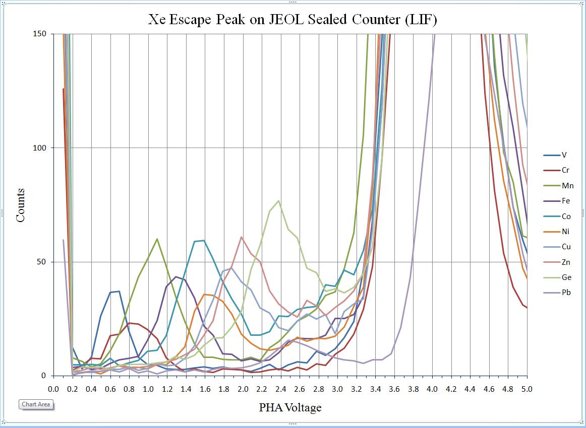
SCA scan for V (JEOL Xe counter, LiF crystal, V metal)
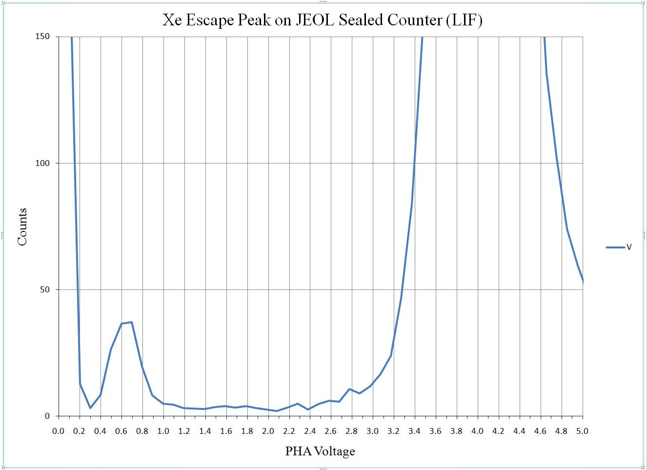
SCA scan for Cr (JEOL Xe counter, LiF crystal, Cr2O3)
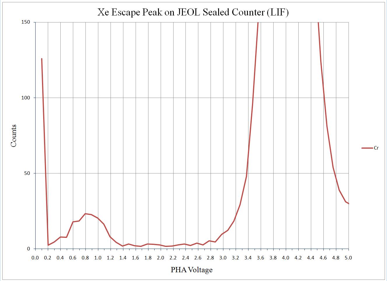
SCA scan for Mn (JEOL Xe counter, LiF crystal, Mn metal)
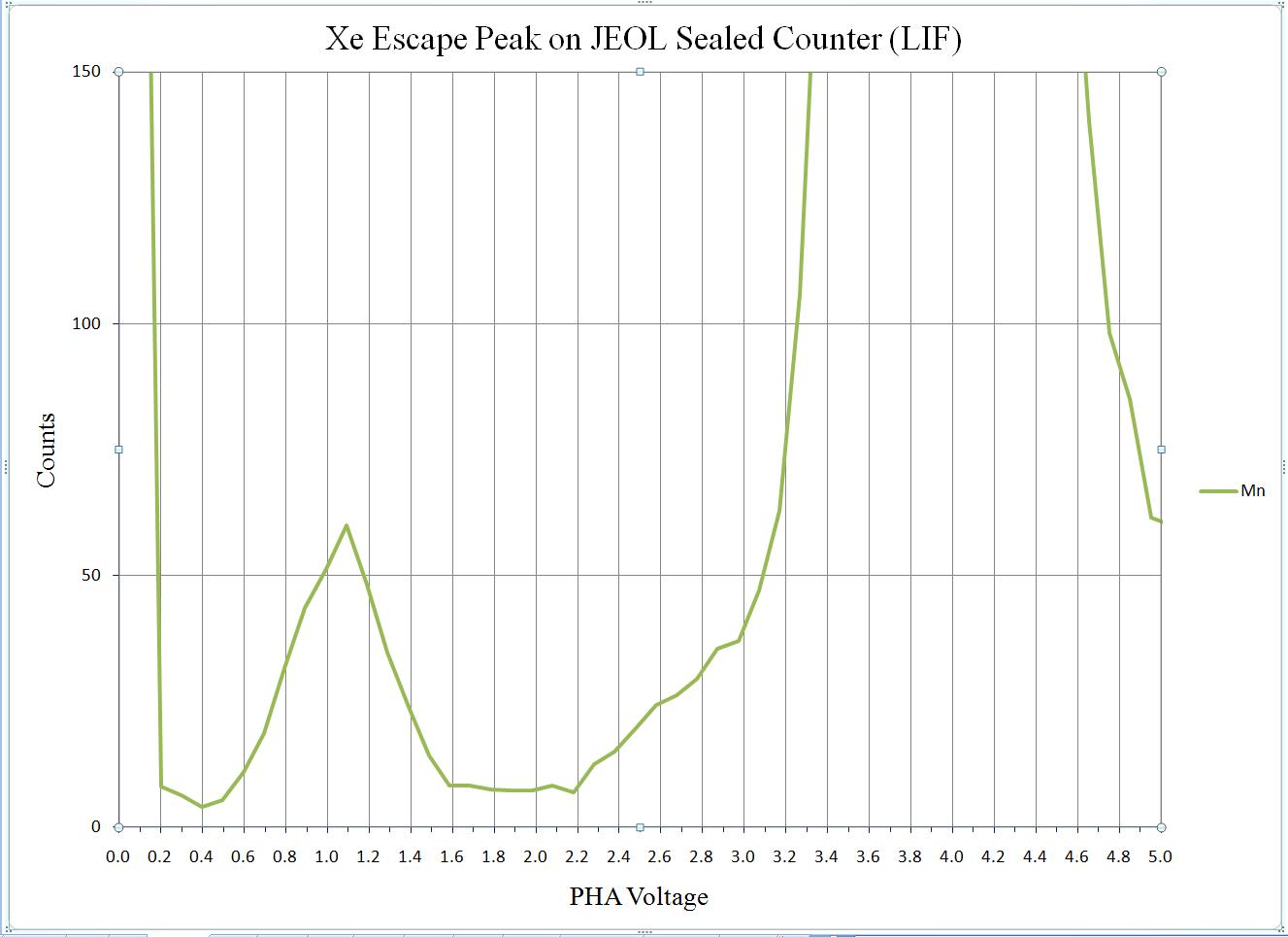
SCA scan for Fe (JEOL Xe counter, LiF crystal, Hematite)
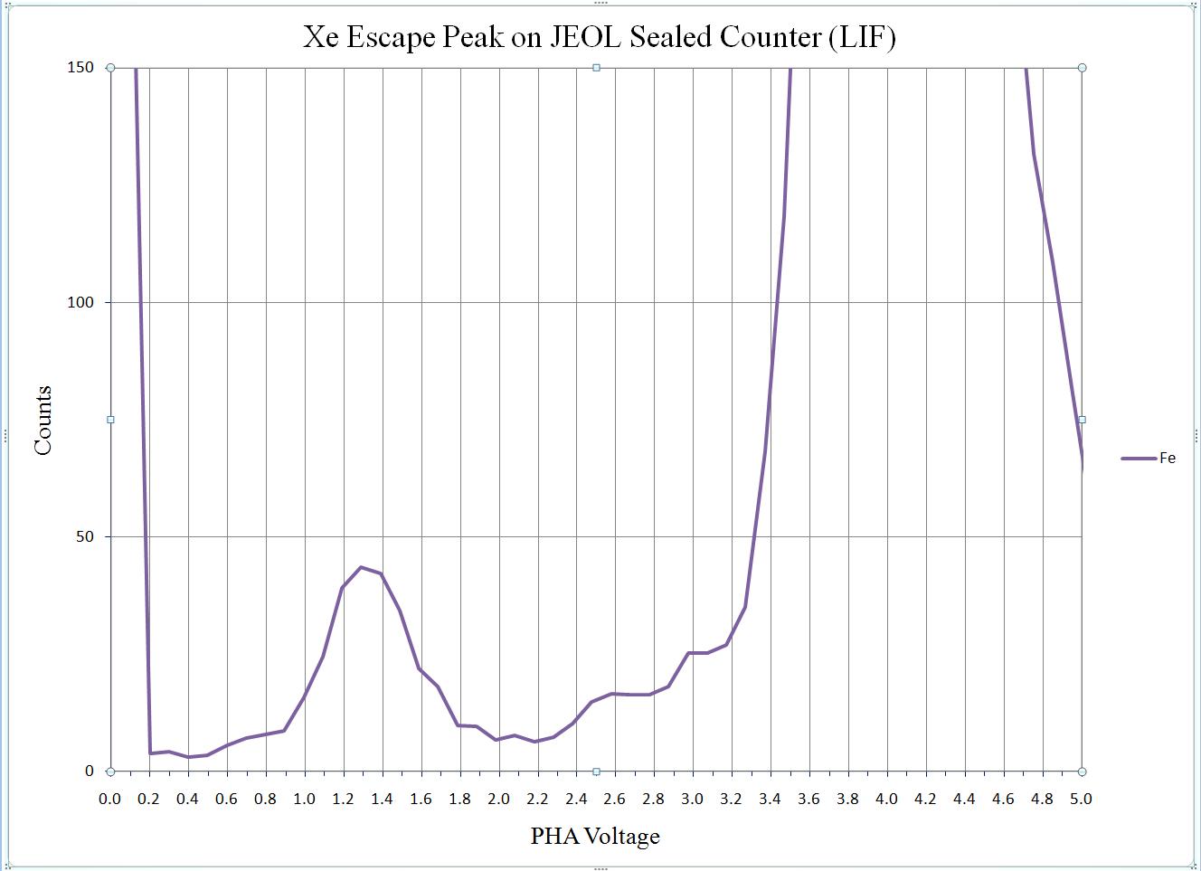
SCA scan for Co (JEOL Xe counter, LiF crystal, Co metal)
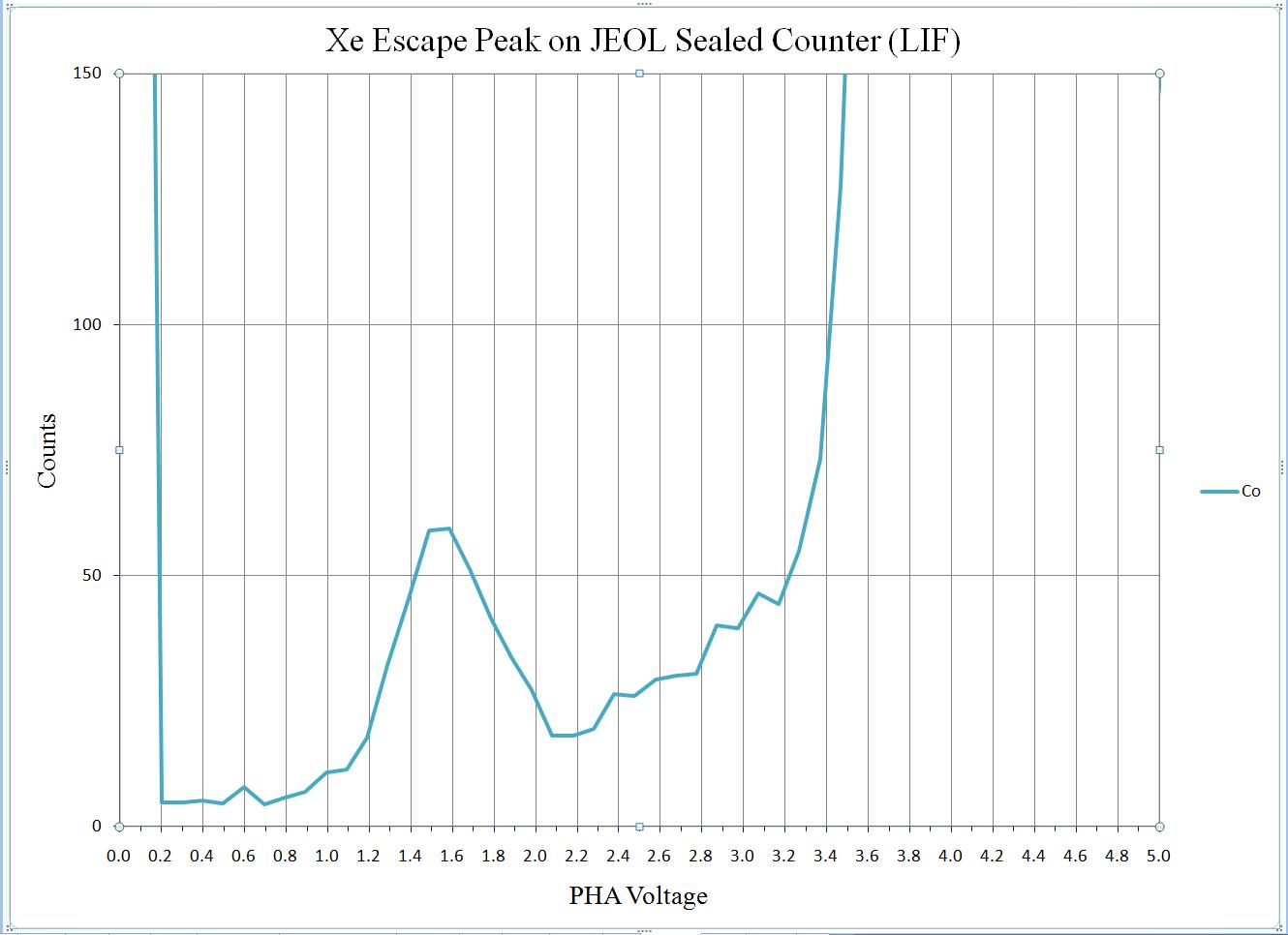
SCA scan for Ni (JEOL Xe counter, LiF crystal, Ni olivine)
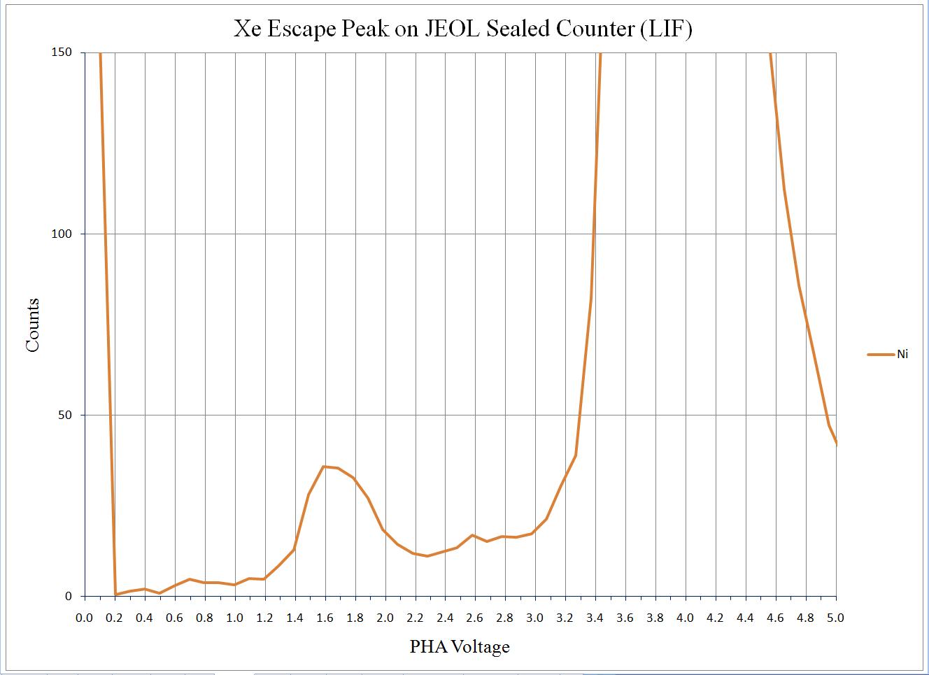
SCA scan for Cu (JEOL Xe counter, LiF crystal, NIST SRM 478 Brass )
SCA scan for Zn (JEOL Xe counter, LiF crystal, Zn metal)
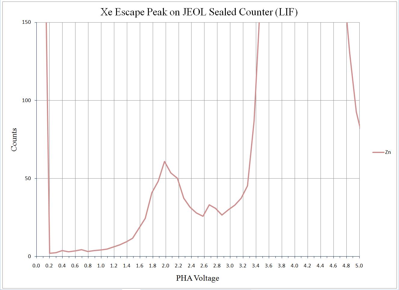
SCA scan for Ge (JEOL Xe counter, LiF crystal, Ge metal)
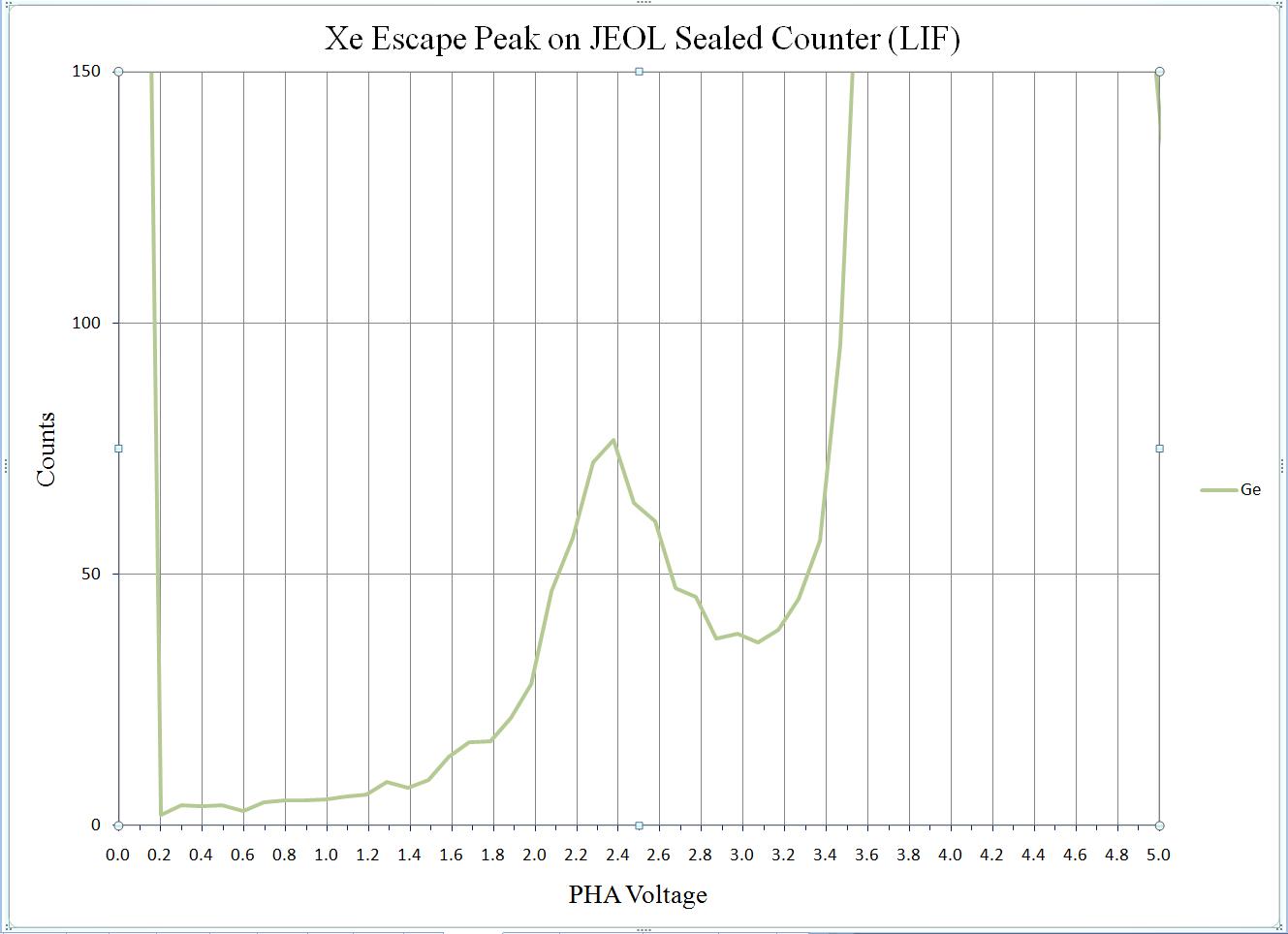
SCA scan for Pb Lα (JEOL Xe counter, LiF crystal, PbS)
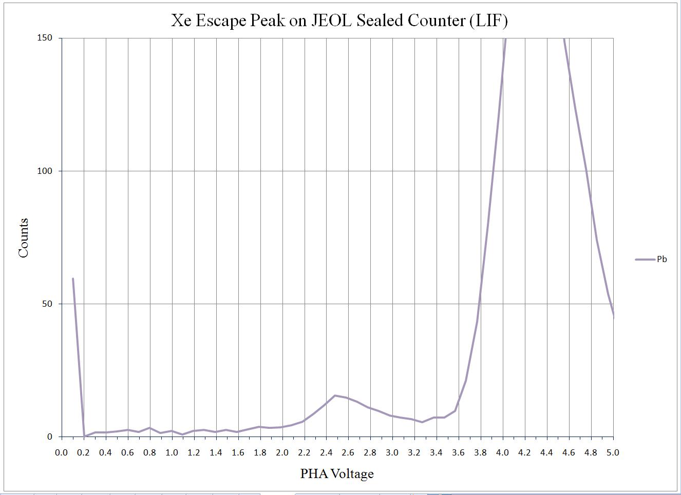
Return to Microanalysis Facility
Page last updated on:
Copyright © Dan Kremser, HTML Paul Carpenter